Debiased Machine Learning — dml • dml.sensemakr

Estimates a target parameter of interest, such as an average treatment effect (ATE), using Debiased Machine #Learning (DML).

The function dml_gate is a convenience function that adds groups to a dml object after the model is fit.

dml(
  y,
  d,
  x,
  model = c("plm", "npm"),
  target = "ate",
  groups = NULL,
  cf.folds = 5,
  cf.reps = 1,
  cf.seed = NULL,
  ps.trim = 0.01,
  reg = "ranger",
  yreg = reg,
  dreg = reg,
  dirty.tuning = TRUE,
  save.models = FALSE,
  y.class = FALSE,
  d.class = FALSE,
  verbose = TRUE,
  warnings = FALSE
)

dml_gate(dml.fit, groups, ...)

Arguments

y: numeric vector with the outcome.
d: numeric vector with the treatment. If the treatment is binary, it needs to be encoded as as: zero = absence of treatment, one = presence of treatment.
x: numeric vector or matrix with covariates. We suggest constructing x using model.matrix.
model: specifies the model. Current available options are plm for a partially linear model, and npm for a fully non-parametric model.
target: specifies the target causal quantity of interest. Available options are ate (ATE - average treatment effect), att (ATT - average treatment effect on the treated), and atu (ATU - average treatment effect on the untreated). Note that for the partially linear model with a continuous treatment the ATE also equals the average causal derivative (ACD). For the nonparametric model, these are only available for binary treatments.
groups: a factor or numeric vector indicating group membership. Groups must be a deterministic function of x.
cf.folds: number of cross-fitting folds. Default is 5.
cf.reps: number of cross-fitting repetitions. Default is 1.
cf.seed: optional integer. A random seed for reproducibility of fold assignments.
ps.trim: trims propensity scores lower than ps.trim and greater than 1-ps.trim, in order to obtain more stable estimates. Alternatively, a named list with elements lower and upper specifying the lower and upper bounds for trimming. This is only relevant for the case of a binary treatment and when model = "npm".
reg: details of the machine learning method to be used for estimating the nuisance parameters (e.g, regression functions of the treatment and the outcome). Currently, this should be specified using the same arguments as caret's train function. The default is random forest using ranger. The default method is fast and usually works well for many applications.
yreg: same as reg, but specifies arguments for the outcome regression alone. Default is the same value of reg. Alternatively, a named list with elements yreg0 and yreg1 specifying separate methods for each.
dreg: same as reg, but specifies arguments for the treatment regression alone. Default is the same value of reg.
dirty.tuning: should the tuning of the machine learning method happen within each cross-fit fold ("clean"), or using all the data ("dirty")? Default is dirty tuning (dirty.tuning = TRUE). As long as the number of choices for the tuning parameters is not too big, dirty tuning is faster and should not affect the asymptotic guarantees of DML.
save.models: should the fitted models of each iterated be saved? Default is FALSE. Note that setting this to true could end up using a lot of memory.
y.class: when y is binary, should the outcome regression be treated as a classification problem? Default is FALSE. Note that for DML we need the class probabilities, and regression gives us that. If you change to classification, you need to make sure the method outputs class probabilities.
d.class: when d is binary, should the outcome regression be treated as a classification problem? Default is FALSE. Note that for DML we need the class probabilities, and regression gives us that. If you change to classification, you need to make sure the method outputs class probabilities.
verbose: if TRUE (default) prints steps of the fitting procedure.
warnings: should caret's warnings be printed? Default is FALSE. Note caret has many inconsistent and unnecessary warnings.
dml.fit: an object of class dml.
...: arguments passed to other methods.

Value

An object of class dml with the results of the DML procedure. The object is a list containing:

data: A list with the data used.
call: The original call used to fit the model.
info: A list with general information and arguments of the DML fitting procedure.
fits: A list with the predictions of each repetition.
results: A list with the results (influence functions and estimates) for each repetition.
coefs: A list with the estimates and standard errors for each repetition.

References

Chernozhukov, V., Cinelli, C., Newey, W., Sharma A., and Syrgkanis, V. (2026). "Long Story Short: Omitted Variable Bias in Causal Machine Learning." Review of Economics and Statistics. doi:10.1162/REST.a.1705

Examples

# loads package
library(dml.sensemakr)

## loads data
data("pension")

# set the outcome
y <- pension$net_tfa  # net total financial assets

# set the treatment
d <- pension$e401    # 401K eligibility

# set the covariates (a matrix)
x <- model.matrix(~ -1 + age + inc  + educ+ fsize + marr + twoearn + pira + hown, data = pension)

## compute income quartiles for group ATE.
g1 <- cut(x[,"inc"], quantile(x[,"inc"], c(0, 0.25,.5,.75,1), na.rm = TRUE),
         labels = c("q1", "q2", "q3", "q4"), include.lowest = TRUE)
# run DML (nonparametric model)
## 2 folds (change as needed)
## 1 repetition (change as needed)
dml.401k <- dml(y, d, x, model = "npm", groups = g1, cf.folds = 2, cf.reps = 1)
#> Debiased Machine Learning
#> 
#>  Model: Nonparametric 
#>  Target: ate 
#>  Cross-Fitting: 2 folds, 1 reps 
#>  ML Method: outcome (yreg0:ranger, yreg1:ranger), treatment (ranger)
#>  Tuning: dirty 
#> 
#> 
#> ====================================
#> Tuning parameters using all the data
#> ====================================
#> 
#> - Tuning Model for D.
#> -- Best Tune:
#>   mtry min.node.size splitrule
#> 1    2             5  variance
#> 
#> - Tuning Model for Y (non-parametric).
#> -- Best Tune:
#>   mtry min.node.size splitrule
#> 1    2             5  variance
#>   mtry min.node.size splitrule
#> 1    2             5  variance
#> 
#> 
#> ======================================
#> Repeating 2-fold cross-fitting 1 times
#> ======================================
#> 
#> -- Rep 1 -- Folds: 1  2  
#> 

# summary of results with median method (default)
summary(dml.401k, combine.method = "median")
#> 
#> Debiased Machine Learning
#> 
#>  Model: Nonparametric 
#>  Cross-Fitting: 2 folds, 1 reps 
#>  ML Method: outcome (yreg0:ranger, yreg1:ranger, R2 = 26.034%), treatment (ranger, R2 = 11.251%)
#>  Tuning: dirty 
#> 
#> Average Treatment Effect: 
#> 
#>         Estimate Std. Error t value P(>|t|)    
#> ate.all     7763       1145   6.781 1.2e-11 ***
#> ---
#> Signif. codes:  0 ‘***’ 0.001 ‘**’ 0.01 ‘*’ 0.05 ‘.’ 0.1 ‘ ’ 1
#> 
#> Group Average Treatment Effect: 
#> 
#>         Estimate Std. Error t value  P(>|t|)    
#> gate.q1     4772        840   5.681 1.34e-08 ***
#> gate.q2     3093       1217   2.541 0.011048 *  
#> gate.q3     6330       1760   3.596 0.000323 ***
#> gate.q4    16854       3955   4.262 2.03e-05 ***
#> ---
#> Signif. codes:  0 ‘***’ 0.001 ‘**’ 0.01 ‘*’ 0.05 ‘.’ 0.1 ‘ ’ 1
#> 
#> Note: DML estimates combined using the median method.
#> 
#> Verbal interpretation of DML procedure:
#> 
#> -- Average treatment effects were estimated using DML with 2-fold cross-fitting. In order to reduce the variance that stems from sample splitting, we repeated the procedure 1 times. Estimates are combined using the median as the final estimate, incorporating variation across experiments into the standard error as described in Chernozhukov et al. (2018). The outcome regression uses  from the R package ; the treatment regression uses Random Forest from the R package ranger.

# coef median method (default)
coef(dml.401k, combine.method = "median")
#>   ate.all   gate.q1   gate.q2   gate.q3   gate.q4 
#>  7762.915  4772.061  3093.195  6330.041 16854.429 

# se median method (default)
se(dml.401k, combine.method = "median")
#>   ate.all   gate.q1   gate.q2   gate.q3   gate.q4 
#> 1144.8702  839.9974 1217.2293 1760.0668 3954.6826 

# confint median method
confint(dml.401k, combine.method = "median")
#>             2.5 %    97.5 %
#> ate.all 5519.0104 10006.819
#> gate.q1 3125.6963  6418.426
#> gate.q2  707.4699  5478.921
#> gate.q3 2880.3735  9779.708
#> gate.q4 9103.3935 24605.465

## Sensitivity Analysis

### Robustness Values
robustness_value(dml.401k, alpha = 0.05)
#>    ate.all    gate.q1    gate.q2    gate.q3    gate.q4 
#> 0.04377913 0.07882806 0.01530738 0.03302966 0.05237003 

### Confidence Bounds
confidence_bounds(dml.401k, cf.y = 0.03, cf.d = 0.04, level = 0.95)
#>                lwr        upr
#> ate.all  1256.9657 14264.6146
#> gate.q1  1951.1698  7711.1079
#> gate.q2 -1451.3430  6982.7950
#> gate.q3  -187.0972 12637.9706
#> gate.q4  3587.5139 30200.0130
#> 
#> Confidence level: point = 95%; region = 90%.
#> Sensitivity parameters: cf.y = 0.03; cf.d = 0.04; rho2 = 1.

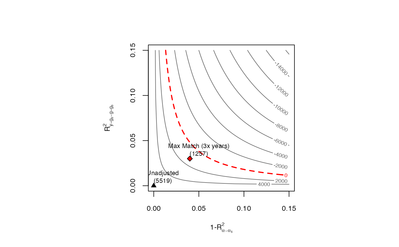
### Contour Plots
ovb_contour_plot(dml.401k, cf.y = 0.03, cf.d = 0.04,
                bound.label = "Max Match (3x years)")