The sensemakr package implements a suite of sensitivity analysis tools that makes it easier to understand the impact of omitted variables in linear regression models, as discussed in Cinelli and Hazlett (2020).
Details
The main function of the package is sensemakr, which computes the most common sensitivity analysis results.
After running sensemakr you may directly use the plot and print methods in the returned object.
You may also use the other sensitivity functions of the package directly, such as the functions for sensitivity plots
(ovb_contour_plot, ovb_extreme_plot) the functions for computing bias-adjusted estimates and t-values (adjusted_estimate, adjusted_t),
the functions for computing the robustness value and partial R2 (robustness_value, partial_r2), or the functions for bounding the strength
of unobserved confounders (ovb_bounds), among others.
More information can be found on the help documentation, vignettes and related papers.
References
Cinelli, C. and Hazlett, C. (2020), "Making Sense of Sensitivity: Extending Omitted Variable Bias." Journal of the Royal Statistical Society, Series B (Statistical Methodology).
See also
Useful links:
Examples
# loads dataset
data("darfur")
# runs regression model
model <- lm(peacefactor ~ directlyharmed + age + farmer_dar + herder_dar +
pastvoted + hhsize_darfur + female + village, data = darfur)
# runs sensemakr for sensitivity analysis
sensitivity <- sensemakr(model, treatment = "directlyharmed",
benchmark_covariates = "female",
kd = 1:3)
# short description of results
sensitivity
#> Sensitivity Analysis to Unobserved Confounding
#>
#> Model Formula: peacefactor ~ directlyharmed + age + farmer_dar + herder_dar +
#> pastvoted + hhsize_darfur + female + village
#>
#> Null hypothesis: q = 1 and reduce = TRUE
#>
#> Observed Estimates of ' directlyharmed ':
#> Coef. estimate: 0.09732
#> Standard Error: 0.02326
#> t-value: 4.18445
#>
#> Sensitivity Statistics:
#> Partial R2 of treatment with outcome: 0.02187
#> Robustness Value, q = 1 : 0.13878
#> Robustness Value, q = 1 alpha = 0.05 : 0.07626
#>
#> For more information, check summary.
# long description of results
summary(sensitivity)
#> Sensitivity Analysis to Unobserved Confounding
#>
#> Model Formula: peacefactor ~ directlyharmed + age + farmer_dar + herder_dar +
#> pastvoted + hhsize_darfur + female + village
#>
#> Null hypothesis: q = 1 and reduce = TRUE
#> -- This means we are considering biases that reduce the absolute value of the current estimate.
#> -- The null hypothesis deemed problematic is H0:tau = 0
#>
#> Observed Estimates of 'directlyharmed':
#> Coef. estimate: 0.0973
#> Standard Error: 0.0233
#> t-value (H0:tau = 0): 4.1844
#>
#> Sensitivity Statistics:
#> Partial R2 of treatment with outcome: 0.0219
#> Robustness Value, q = 1: 0.1388
#> Robustness Value, q = 1, alpha = 0.05: 0.0763
#>
#> Verbal interpretation of sensitivity statistics:
#>
#> -- Partial R2 of the treatment with the outcome: an extreme confounder (orthogonal to the covariates) that explains 100% of the residual variance of the outcome, would need to explain at least 2.19% of the residual variance of the treatment to fully account for the observed estimated effect.
#>
#> -- Robustness Value, q = 1: unobserved confounders (orthogonal to the covariates) that explain more than 13.88% of the residual variance of both the treatment and the outcome are strong enough to bring the point estimate to 0 (a bias of 100% of the original estimate). Conversely, unobserved confounders that do not explain more than 13.88% of the residual variance of both the treatment and the outcome are not strong enough to bring the point estimate to 0.
#>
#> -- Robustness Value, q = 1, alpha = 0.05: unobserved confounders (orthogonal to the covariates) that explain more than 7.63% of the residual variance of both the treatment and the outcome are strong enough to bring the estimate to a range where it is no longer 'statistically different' from 0 (a bias of 100% of the original estimate), at the significance level of alpha = 0.05. Conversely, unobserved confounders that do not explain more than 7.63% of the residual variance of both the treatment and the outcome are not strong enough to bring the estimate to a range where it is no longer 'statistically different' from 0, at the significance level of alpha = 0.05.
#>
#> Bounds on omitted variable bias:
#>
#> --The table below shows the maximum strength of unobserved confounders with association with the treatment and the outcome bounded by a multiple of the observed explanatory power of the chosen benchmark covariate(s).
#>
#> Bound Label R2dz.x R2yz.dx Treatment Adjusted Estimate Adjusted Se
#> 1x female 0.0092 0.1246 directlyharmed 0.0752 0.0219
#> 2x female 0.0183 0.2493 directlyharmed 0.0529 0.0204
#> 3x female 0.0275 0.3741 directlyharmed 0.0304 0.0187
#> Adjusted T Adjusted Lower CI Adjusted Upper CI
#> 3.4389 0.0323 0.1182
#> 2.6002 0.0130 0.0929
#> 1.6281 -0.0063 0.0670
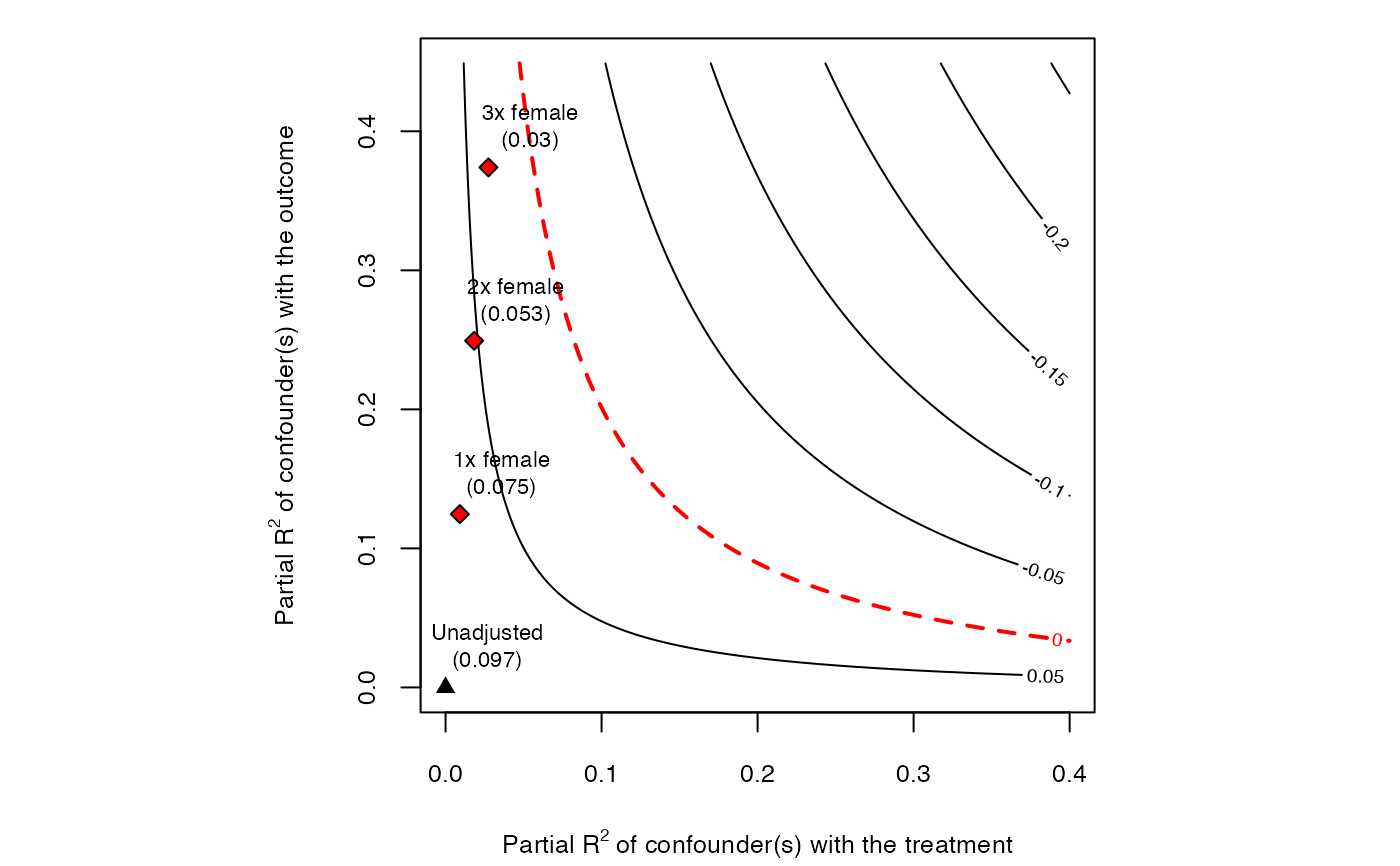
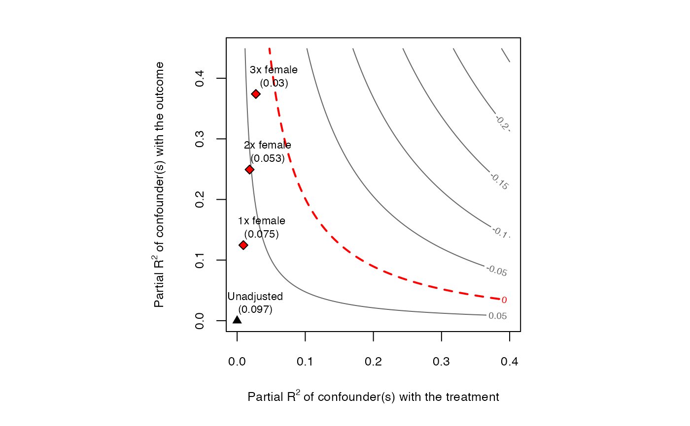
# plot bias contour of point estimate
plot(sensitivity)
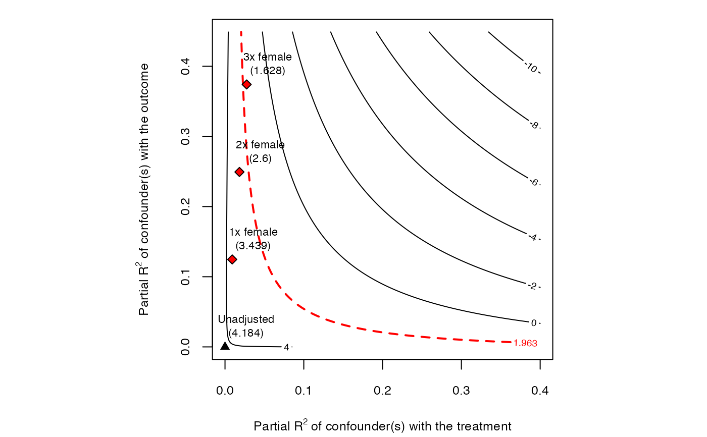
 # plot bias contour of t-value
plot(sensitivity, sensitivity.of = "t-value")
# plot bias contour of t-value
plot(sensitivity, sensitivity.of = "t-value")
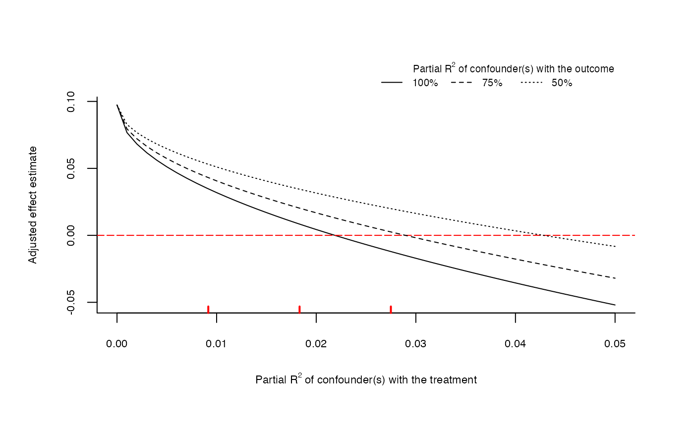
 # plot extreme scenario
plot(sensitivity, type = "extreme")
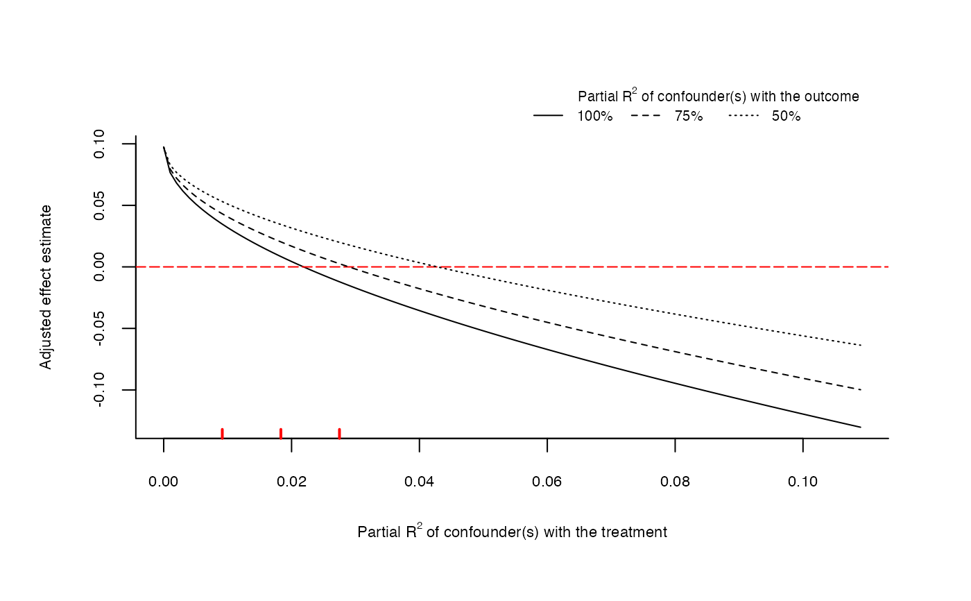
# plot extreme scenario
plot(sensitivity, type = "extreme")
 # latex code for sensitivity table
ovb_minimal_reporting(sensitivity)
#> \begin{table}[!h]
#> \centering
#> \begin{tabular}{lrrrrrr}
#> \multicolumn{7}{c}{Outcome: \textit{peacefactor}} \\
#> \hline \hline
#> Treatment: & Est. & S.E. & t-value & $R^2_{Y \sim D |{\bf X}}$ & $RV_{q = 1}$ & $RV_{q = 1, \alpha = 0.05}$ \\
#> \hline
#> \textit{directlyharmed} & 0.097 & 0.023 & 4.184 & 2.2\% & 13.9\% & 7.6\% \\
#> \hline
#> df = 783 & & \multicolumn{5}{r}{ \small \textit{Bound (1x female)}: $R^2_{Y\sim Z| {\bf X}, D}$ = 12.5\%, $R^2_{D\sim Z| {\bf X} }$ = 0.9\%} \\
#> \end{tabular}
#> \end{table}
# data.frame with sensitivity statistics
sensitivity$sensitivity_stats
#> treatment estimate se t_statistic r2yd.x rv_q
#> 1 directlyharmed 0.09731582 0.02325654 4.18445 0.02187309 0.1387764
#> rv_qa f2yd.x dof
#> 1 0.07625797 0.02236222 783
# data.frame with bounds on the strengh of confounders
sensitivity$bounds
#> bound_label r2dz.x r2yz.dx treatment adjusted_estimate
#> 1 1x female 0.009164287 0.1246409 directlyharmed 0.07522027
#> 2 2x female 0.018328573 0.2493241 directlyharmed 0.05291517
#> 3 3x female 0.027492860 0.3740505 directlyharmed 0.03039602
#> adjusted_se adjusted_t adjusted_lower_CI adjusted_upper_CI
#> 1 0.02187333 3.438904 0.032282966 0.11815758
#> 2 0.02035006 2.600246 0.012968035 0.09286231
#> 3 0.01867006 1.628062 -0.006253282 0.06704533
### Using sensitivity functions directly ###
# robustness value of directly harmed q = 1 (reduce estimate to zero)
robustness_value(model, covariates = "directlyharmed")
#> directlyharmed
#> 0.0763
#> Parameters: q = 1, alpha = 0.05, invert = FALSE
# robustness value of directly harmed q = 1/2 (reduce estimate in half)
robustness_value(model, covariates = "directlyharmed", q = 1/2)
#> directlyharmed
#> 0.00456
#> Parameters: q = 0.5, alpha = 0.05, invert = FALSE
# robustness value of directly harmed q = 1/2, alpha = 0.05
robustness_value(model, covariates = "directlyharmed", q = 1/2, alpha = 0.05)
#> directlyharmed
#> 0.00456
#> Parameters: q = 0.5, alpha = 0.05, invert = FALSE
# partial R2 of directly harmed with peacefactor
partial_r2(model, covariates = "directlyharmed")
#> directlyharmed
#> 0.02187309
# partial R2 of female with peacefactor
partial_r2(model, covariates = "female")
#> female
#> 0.1090339
# data.frame with sensitivity statistics
sensitivity_stats(model, treatment = "directlyharmed")
#> treatment estimate se t_statistic r2yd.x rv_q
#> 1 directlyharmed 0.09731582 0.02325654 4.18445 0.02187309 0.1387764
#> rv_qa f2yd.x dof
#> 1 0.07625797 0.02236222 783
# bounds on the strength of confounders using female and age
ovb_bounds(model,
treatment = "directlyharmed",
benchmark_covariates = c("female", "age"),
kd = 1:3)
#> bound_label r2dz.x r2yz.dx treatment adjusted_estimate
#> 1 1x female 0.009164287 0.124640923 directlyharmed 0.07522027
#> 2 2x female 0.018328573 0.249324064 directlyharmed 0.05291517
#> 3 3x female 0.027492860 0.374050471 directlyharmed 0.03039602
#> 4 1x age 0.001117013 0.008107259 directlyharmed 0.09535637
#> 5 2x age 0.002234026 0.016214559 directlyharmed 0.09339472
#> 6 3x age 0.003351038 0.024321900 directlyharmed 0.09143086
#> adjusted_se adjusted_t adjusted_lower_CI adjusted_upper_CI
#> 1 0.02187333 3.438904 0.032282966 0.11815758
#> 2 0.02035006 2.600246 0.012968035 0.09286231
#> 3 0.01867006 1.628062 -0.006253282 0.06704533
#> 4 0.02318983 4.111990 0.049834764 0.14087797
#> 5 0.02310779 4.041698 0.048034163 0.13875527
#> 6 0.02302527 3.970892 0.046232296 0.13662943
# adjusted estimate given hypothetical strength of confounder
adjusted_estimate(model, treatment = "directlyharmed", r2dz.x = 0.1, r2yz.dx = 0.1)
#> directlyharmed
#> 0.02871889
# adjusted t-value given hypothetical strength of confounder
adjusted_t(model, treatment = "directlyharmed", r2dz.x = 0.1, r2yz.dx = 0.1)
#> [1] 1.234085
#> H0:tau = 0
# bias contour plot directly from lm model
ovb_contour_plot(model,
treatment = "directlyharmed",
benchmark_covariates = "female",
kd = 1:3)
# latex code for sensitivity table
ovb_minimal_reporting(sensitivity)
#> \begin{table}[!h]
#> \centering
#> \begin{tabular}{lrrrrrr}
#> \multicolumn{7}{c}{Outcome: \textit{peacefactor}} \\
#> \hline \hline
#> Treatment: & Est. & S.E. & t-value & $R^2_{Y \sim D |{\bf X}}$ & $RV_{q = 1}$ & $RV_{q = 1, \alpha = 0.05}$ \\
#> \hline
#> \textit{directlyharmed} & 0.097 & 0.023 & 4.184 & 2.2\% & 13.9\% & 7.6\% \\
#> \hline
#> df = 783 & & \multicolumn{5}{r}{ \small \textit{Bound (1x female)}: $R^2_{Y\sim Z| {\bf X}, D}$ = 12.5\%, $R^2_{D\sim Z| {\bf X} }$ = 0.9\%} \\
#> \end{tabular}
#> \end{table}
# data.frame with sensitivity statistics
sensitivity$sensitivity_stats
#> treatment estimate se t_statistic r2yd.x rv_q
#> 1 directlyharmed 0.09731582 0.02325654 4.18445 0.02187309 0.1387764
#> rv_qa f2yd.x dof
#> 1 0.07625797 0.02236222 783
# data.frame with bounds on the strengh of confounders
sensitivity$bounds
#> bound_label r2dz.x r2yz.dx treatment adjusted_estimate
#> 1 1x female 0.009164287 0.1246409 directlyharmed 0.07522027
#> 2 2x female 0.018328573 0.2493241 directlyharmed 0.05291517
#> 3 3x female 0.027492860 0.3740505 directlyharmed 0.03039602
#> adjusted_se adjusted_t adjusted_lower_CI adjusted_upper_CI
#> 1 0.02187333 3.438904 0.032282966 0.11815758
#> 2 0.02035006 2.600246 0.012968035 0.09286231
#> 3 0.01867006 1.628062 -0.006253282 0.06704533
### Using sensitivity functions directly ###
# robustness value of directly harmed q = 1 (reduce estimate to zero)
robustness_value(model, covariates = "directlyharmed")
#> directlyharmed
#> 0.0763
#> Parameters: q = 1, alpha = 0.05, invert = FALSE
# robustness value of directly harmed q = 1/2 (reduce estimate in half)
robustness_value(model, covariates = "directlyharmed", q = 1/2)
#> directlyharmed
#> 0.00456
#> Parameters: q = 0.5, alpha = 0.05, invert = FALSE
# robustness value of directly harmed q = 1/2, alpha = 0.05
robustness_value(model, covariates = "directlyharmed", q = 1/2, alpha = 0.05)
#> directlyharmed
#> 0.00456
#> Parameters: q = 0.5, alpha = 0.05, invert = FALSE
# partial R2 of directly harmed with peacefactor
partial_r2(model, covariates = "directlyharmed")
#> directlyharmed
#> 0.02187309
# partial R2 of female with peacefactor
partial_r2(model, covariates = "female")
#> female
#> 0.1090339
# data.frame with sensitivity statistics
sensitivity_stats(model, treatment = "directlyharmed")
#> treatment estimate se t_statistic r2yd.x rv_q
#> 1 directlyharmed 0.09731582 0.02325654 4.18445 0.02187309 0.1387764
#> rv_qa f2yd.x dof
#> 1 0.07625797 0.02236222 783
# bounds on the strength of confounders using female and age
ovb_bounds(model,
treatment = "directlyharmed",
benchmark_covariates = c("female", "age"),
kd = 1:3)
#> bound_label r2dz.x r2yz.dx treatment adjusted_estimate
#> 1 1x female 0.009164287 0.124640923 directlyharmed 0.07522027
#> 2 2x female 0.018328573 0.249324064 directlyharmed 0.05291517
#> 3 3x female 0.027492860 0.374050471 directlyharmed 0.03039602
#> 4 1x age 0.001117013 0.008107259 directlyharmed 0.09535637
#> 5 2x age 0.002234026 0.016214559 directlyharmed 0.09339472
#> 6 3x age 0.003351038 0.024321900 directlyharmed 0.09143086
#> adjusted_se adjusted_t adjusted_lower_CI adjusted_upper_CI
#> 1 0.02187333 3.438904 0.032282966 0.11815758
#> 2 0.02035006 2.600246 0.012968035 0.09286231
#> 3 0.01867006 1.628062 -0.006253282 0.06704533
#> 4 0.02318983 4.111990 0.049834764 0.14087797
#> 5 0.02310779 4.041698 0.048034163 0.13875527
#> 6 0.02302527 3.970892 0.046232296 0.13662943
# adjusted estimate given hypothetical strength of confounder
adjusted_estimate(model, treatment = "directlyharmed", r2dz.x = 0.1, r2yz.dx = 0.1)
#> directlyharmed
#> 0.02871889
# adjusted t-value given hypothetical strength of confounder
adjusted_t(model, treatment = "directlyharmed", r2dz.x = 0.1, r2yz.dx = 0.1)
#> [1] 1.234085
#> H0:tau = 0
# bias contour plot directly from lm model
ovb_contour_plot(model,
treatment = "directlyharmed",
benchmark_covariates = "female",
kd = 1:3)
 # extreme scenario plot directly from lm model
ovb_extreme_plot(model,
treatment = "directlyharmed",
benchmark_covariates = "female",
kd = 1:3, lim = 0.05)
# extreme scenario plot directly from lm model
ovb_extreme_plot(model,
treatment = "directlyharmed",
benchmark_covariates = "female",
kd = 1:3, lim = 0.05)