Here we reproduce the empirical example of Chernozhukov, V., Cinelli, C., Newey, W., Sharma A., and Syrgkanis, V. (2026). “Long Story Short: Omitted Variable Bias in Causal Machine Learning.” Review of Economics and Statistics.
Load Data
# loads package
library(dml.sensemakr)

## loads data
data("pension")
y <- pension$net_tfa # net total financial assets
d <- pension$e401 # 401K eligibility
x <- model.matrix(~ -1 + age + inc + educ+ fsize + marr + twoearn + pira + hown, data = pension)Partially Linear Model
# run DML
dml.401k.plm <- dml(y, d, x, model = "plm", cf.folds = 5, cf.reps = 5)
#> Debiased Machine Learning
#>
#>  Model: Partially Linear
#>  Target: ate
#>  Cross-Fitting: 5 folds, 5 reps
#>  ML Method: outcome (yreg0:ranger, yreg1:ranger), treatment (ranger)
#>  Tuning: dirty
#>
#>
#> ====================================
#> Tuning parameters using all the data
#> ====================================
#>
#> - Tuning Model for D.
#> -- Best Tune:
#>   mtry min.node.size splitrule
#> 1    2             5  variance
#>
#> - Tuning Model for Y (partially linear).
#> -- Best Tune:
#>   mtry min.node.size splitrule
#> 1    2             5  variance
#>
#>
#> ======================================
#> Repeating 5-fold cross-fitting 5 times
#> ======================================
#>
#> -- Rep 1 -- Folds: 1  2  3  4  5
#>
#> -- Rep 2 -- Folds: 1  2  3  4  5
#>
#> -- Rep 3 -- Folds: 1  2  3  4  5
#>
#> -- Rep 4 -- Folds: 1  2  3  4  5
#>
#> -- Rep 5 -- Folds: 1  2  3  4  5
# results under conditional ignorability
summary(dml.401k.plm)
#>
#> Debiased Machine Learning
#>
#>  Model: Partially Linear
#>  Cross-Fitting: 5 folds, 5 reps
#>  ML Method: outcome (yreg0:ranger, yreg1:ranger, R2 = 27.302%), treatment (ranger, R2 = 11.612%)
#>  Tuning: dirty
#>
#> Average Treatment Effect:
#>
#>         Estimate Std. Error t value  P(>|t|)
#> ate.all     9018       1315    6.86 6.89e-12 ***
#> ---
#> Signif. codes:  0 '***' 0.001 '**' 0.01 '*' 0.05 '.' 0.1 ' ' 1
#> Note: DML estimates combined using the median method.
#>
#> Verbal interpretation of DML procedure:
#>
#> -- Average treatment effects were estimated using DML with 5-fold cross-fitting. In order to reduce the variance that stems from sample splitting, we repeated the procedure 5 times. Estimates are combined using the median as the final estimate, incorporating variation across experiments into the standard error as described in Chernozhukov et al. (2018). The outcome regression uses  from the R package ; the treatment regression uses Random Forest from the R package ranger.
# sensitivity analysis
sens.401k <- sensemakr(dml.401k.plm, cf.y = 0.04, cf.d = 0.03,)

# summary
summary(sens.401k)
#> ==== Original Analysis ====
#>
#> Debiased Machine Learning
#>
#>  Model: Partially Linear
#>  Cross-Fitting: 5 folds, 5 reps
#>  ML Method: outcome (yreg0:ranger, yreg1:ranger, R2 = 27.302%), treatment (ranger, R2 = 11.612%)
#>  Tuning: dirty
#>
#> Average Treatment Effect:
#>
#>         Estimate Std. Error t value  P(>|t|)
#> ate.all     9018       1315    6.86 6.89e-12 ***
#> ---
#> Signif. codes:  0 '***' 0.001 '**' 0.01 '*' 0.05 '.' 0.1 ' ' 1
#> Note: DML estimates combined using the median method.
#>
#> Verbal interpretation of DML procedure:
#>
#> -- Average treatment effects were estimated using DML with 5-fold cross-fitting. In order to reduce the variance that stems from sample splitting, we repeated the procedure 5 times. Estimates are combined using the median as the final estimate, incorporating variation across experiments into the standard error as described in Chernozhukov et al. (2018). The outcome regression uses  from the R package ; the treatment regression uses Random Forest from the R package ranger.
#>
#> ==== Sensitivity Analysis ====
#>
#> Null hypothesis: theta = 0
#> Signif. level: alpha = 0.05
#>
#> Robustness Values:
#>         RV (%) RVa (%)
#> ate.all 7.3079    5.53
#>
#> Verbal interpretation of robustness values:
#>
#> -- Robustness Value for the Bound (RV): omitted variables that explain more than RV% of the residual variation both of the treatment (cf.d) and of the outcome (cf.y) are sufficiently strong to make the estimated bounds include 0. Conversely, omitted variables that do not explain more than RV% of the residual variation of both the treatment and the outcome are not sufficiently strong to do so.
#>
#> -- Robustness Value for the Confidence Bound (RVa): omitted variables that explain more than RV% of the residual variation both of the treatment (cf.d) and of the outcome (cf.y) are sufficiently strong to make the confidence bounds include 0, at the  significance level of alpha = 0.05. Conversely, omitted variables that do not explain more than RV% of the residual variation of both the treatment and the outcome are not sufficiently strong to do so.
#>
#> Confidence Bounds for Sensitivity Scenario:
#>               lwr       upr
#> ate.all  2651.094 15447.489
#>
#> Confidence level: point = 95%; region = 90%.
#> Sensitivity parameters: cf.y = 0.04; cf.d = 0.03; rho2 = 1.
#>
#> Verbal interpretation of confidence bounds:
#>
#> -- The table shows the lower (lwr) and upper (upr) limits of the confidence bounds on the target quantity, considering omitted variables with postulated sensitivity parameters cf.y, cf.d and rho2. The confidence level "point" is the relevant coverage for most use cases, and stands for the coverage rate for the true target quantity. The confidence level "region" stands for the coverage rate of the true bounds.

# contour plots
oldpar <- par(mfrow = c(1,2))
plot(sens.401k, which.bound = "lwr", bound.label = "Max match (3 years)", col.contour = "blue")
plot(sens.401k, which.bound = "upr", bound.label = "Max match (3 years)", col.contour = "blue")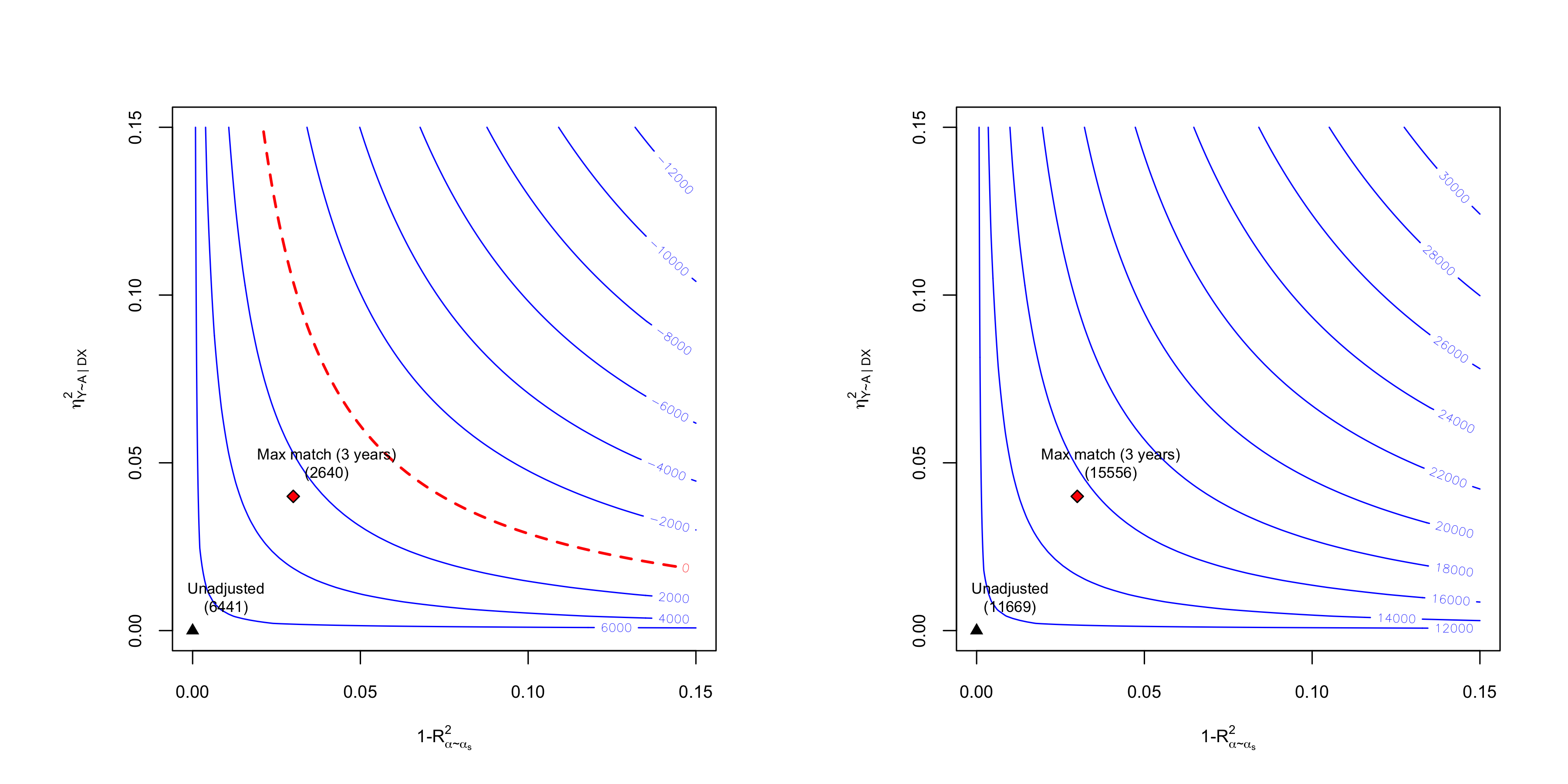
par(oldpar)
# benchmarks
bench.plm <- dml_benchmark(dml.401k.plm, benchmark_covariates = c("inc", "pira", "twoearn"))
#>
#> === Computing benchmarks using covariate: inc  ===
#>
#> Debiased Machine Learning
#>
#>  Model: Partially Linear
#>  Target: ate
#>  Cross-Fitting: 5 folds, 5 reps
#>  ML Method: outcome (yreg0:ranger, yreg1:ranger), treatment (ranger)
#>  Tuning: dirty
#>
#>
#> ====================================
#> Tuning parameters using all the data
#> ====================================
#>
#> - Tuning Model for D.
#> -- Best Tune:
#>   mtry min.node.size splitrule
#> 1    2             5  variance
#>
#> - Tuning Model for Y (partially linear).
#> -- Best Tune:
#>   mtry min.node.size splitrule
#> 1    2             5  variance
#>
#>
#> ======================================
#> Repeating 5-fold cross-fitting 5 times
#> ======================================
#>
#> -- Rep 1 -- Folds: 1  2  3  4  5
#>
#> -- Rep 2 -- Folds: 1  2  3  4  5
#>
#> -- Rep 3 -- Folds: 1  2  3  4  5
#>
#> -- Rep 4 -- Folds: 1  2  3  4  5
#>
#> -- Rep 5 -- Folds: 1  2  3  4  5
#>
#>
#> === Computing benchmarks using covariate: pira  ===
#>
#> Debiased Machine Learning
#>
#>  Model: Partially Linear
#>  Target: ate
#>  Cross-Fitting: 5 folds, 5 reps
#>  ML Method: outcome (yreg0:ranger, yreg1:ranger), treatment (ranger)
#>  Tuning: dirty
#>
#>
#> ====================================
#> Tuning parameters using all the data
#> ====================================
#>
#> - Tuning Model for D.
#> -- Best Tune:
#>   mtry min.node.size splitrule
#> 1    2             5  variance
#>
#> - Tuning Model for Y (partially linear).
#> -- Best Tune:
#>   mtry min.node.size splitrule
#> 1    2             5  variance
#>
#>
#> ======================================
#> Repeating 5-fold cross-fitting 5 times
#> ======================================
#>
#> -- Rep 1 -- Folds: 1  2  3  4  5
#>
#> -- Rep 2 -- Folds: 1  2  3  4  5
#>
#> -- Rep 3 -- Folds: 1  2  3  4  5
#>
#> -- Rep 4 -- Folds: 1  2  3  4  5
#>
#> -- Rep 5 -- Folds: 1  2  3  4  5
#>
#>
#> === Computing benchmarks using covariate: twoearn  ===
#>
#> Debiased Machine Learning
#>
#>  Model: Partially Linear
#>  Target: ate
#>  Cross-Fitting: 5 folds, 5 reps
#>  ML Method: outcome (yreg0:ranger, yreg1:ranger), treatment (ranger)
#>  Tuning: dirty
#>
#>
#> ====================================
#> Tuning parameters using all the data
#> ====================================
#>
#> - Tuning Model for D.
#> -- Best Tune:
#>   mtry min.node.size splitrule
#> 1    2             5  variance
#>
#> - Tuning Model for Y (partially linear).
#> -- Best Tune:
#>   mtry min.node.size splitrule
#> 1    2             5  variance
#>
#>
#> ======================================
#> Repeating 5-fold cross-fitting 5 times
#> ======================================
#>
#> -- Rep 1 -- Folds: 1  2  3  4  5
#>
#> -- Rep 2 -- Folds: 1  2  3  4  5
#>
#> -- Rep 3 -- Folds: 1  2  3  4  5
#>
#> -- Rep 4 -- Folds: 1  2  3  4  5
#>
#> -- Rep 5 -- Folds: 1  2  3  4  5
bench.plm
#>          gain.Y   gain.D     rho theta.s theta.sj  delta
#> inc     0.15441 0.048662  0.3252    9026    12294 3268.0
#> pira    0.05107 0.003184  0.2103    9026     9253  227.0
#> twoearn 0.03817 0.006591 -0.4879    9026     8198 -828.1
Nonparametric Model
## compute income quartiles
g1 <- cut(x[,"inc"], quantile(x[,"inc"], c(0, 0.25,.5,.75,1), na.rm = TRUE),
          labels = c("q1", "q2", "q3", "q4"), include.lowest = TRUE)

## Nonparametric model
dml.401k.npm <- dml(y, d, x, groups = g1, model = "npm", cf.folds = 5, cf.reps = 5)
#> Debiased Machine Learning
#>
#>  Model: Nonparametric
#>  Target: ate
#>  Cross-Fitting: 5 folds, 5 reps
#>  ML Method: outcome (yreg0:ranger, yreg1:ranger), treatment (ranger)
#>  Tuning: dirty
#>
#>
#> ====================================
#> Tuning parameters using all the data
#> ====================================
#>
#> - Tuning Model for D.
#> -- Best Tune:
#>   mtry min.node.size splitrule
#> 1    2             5  variance
#>
#> - Tuning Model for Y (non-parametric).
#> -- Best Tune:
#>   mtry min.node.size splitrule
#> 1    2             5  variance
#>   mtry min.node.size splitrule
#> 1    2             5  variance
#>
#>
#> ======================================
#> Repeating 5-fold cross-fitting 5 times
#> ======================================
#>
#> -- Rep 1 -- Folds: 1  2  3  4  5
#>
#> -- Rep 2 -- Folds: 1  2  3  4  5
#>
#> -- Rep 3 -- Folds: 1  2  3  4  5
#>
#> -- Rep 4 -- Folds: 1  2  3  4  5
#>
#> -- Rep 5 -- Folds: 1  2  3  4  5
# results under conditional ignorability
summary(dml.401k.npm)
#>
#> Debiased Machine Learning
#>
#>  Model: Nonparametric
#>  Cross-Fitting: 5 folds, 5 reps
#>  ML Method: outcome (yreg0:ranger, yreg1:ranger, R2 = 26.613%), treatment (ranger, R2 = 11.487%)
#>  Tuning: dirty
#>
#> Average Treatment Effect:
#>
#>         Estimate Std. Error t value  P(>|t|)
#> ate.all     7898       1218   6.482 9.06e-11 ***
#> ---
#> Signif. codes:  0 '***' 0.001 '**' 0.01 '*' 0.05 '.' 0.1 ' ' 1
#>
#> Group Average Treatment Effect:
#>
#>         Estimate Std. Error t value  P(>|t|)
#> gate.q1   4516.9      851.9   5.302 1.14e-07 ***
#> gate.q2   2529.4     1415.8   1.787 0.074006 .
#> gate.q3   6805.5     1856.9   3.665 0.000247 ***
#> gate.q4  18005.4     4149.1   4.340 1.43e-05 ***
#> ---
#> Signif. codes:  0 '***' 0.001 '**' 0.01 '*' 0.05 '.' 0.1 ' ' 1
#>
#> Note: DML estimates combined using the median method.
#>
#> Verbal interpretation of DML procedure:
#>
#> -- Average treatment effects were estimated using DML with 5-fold cross-fitting. In order to reduce the variance that stems from sample splitting, we repeated the procedure 5 times. Estimates are combined using the median as the final estimate, incorporating variation across experiments into the standard error as described in Chernozhukov et al. (2018). The outcome regression uses  from the R package ; the treatment regression uses Random Forest from the R package ranger.
# load ggplot2
library(ggplot2)

# coefficient plot under conditional ignorability
group.names <- paste0("gate.q",1:4)
df   <- data.frame(groups = 1:4, estimate = coef(dml.401k.npm)[group.names])
cis  <- confint(dml.401k.npm)[group.names, ]
cis  <- setNames(as.data.frame(cis), c("lwr.ci", "upr.ci"))
df   <- cbind(df, cis)
ggplot(df, aes(x = groups, y = estimate)) + geom_line() +
  geom_ribbon(aes(ymin = lwr.ci, ymax = upr.ci), alpha = 0.1, col = "blue", fill = "blue") +
  theme_bw() +
  xlab("Income Groups by Quartiles") +
  ylab("ATE")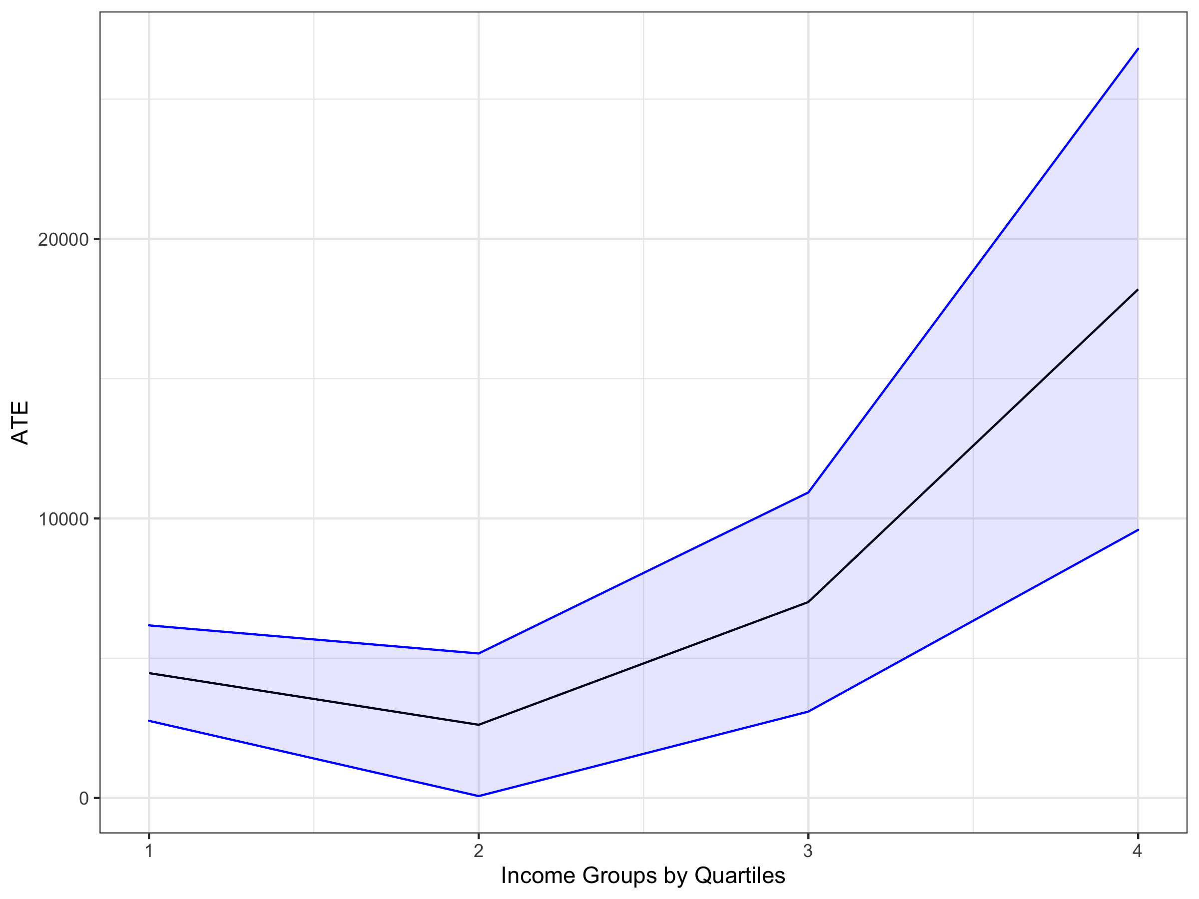
# sensitivity analysis
sens.401k.npm <- sensemakr(dml.401k.npm, cf.y = 0.04, cf.d = 0.03)

# summary
summary(sens.401k.npm)
#> ==== Original Analysis ====
#>
#> Debiased Machine Learning
#>
#>  Model: Nonparametric
#>  Cross-Fitting: 5 folds, 5 reps
#>  ML Method: outcome (yreg0:ranger, yreg1:ranger, R2 = 26.613%), treatment (ranger, R2 = 11.487%)
#>  Tuning: dirty
#>
#> Average Treatment Effect:
#>
#>         Estimate Std. Error t value  P(>|t|)
#> ate.all     7898       1218   6.482 9.06e-11 ***
#> ---
#> Signif. codes:  0 '***' 0.001 '**' 0.01 '*' 0.05 '.' 0.1 ' ' 1
#>
#> Group Average Treatment Effect:
#>
#>         Estimate Std. Error t value  P(>|t|)
#> gate.q1   4516.9      851.9   5.302 1.14e-07 ***
#> gate.q2   2529.4     1415.8   1.787 0.074006 .
#> gate.q3   6805.5     1856.9   3.665 0.000247 ***
#> gate.q4  18005.4     4149.1   4.340 1.43e-05 ***
#> ---
#> Signif. codes:  0 '***' 0.001 '**' 0.01 '*' 0.05 '.' 0.1 ' ' 1
#>
#> Note: DML estimates combined using the median method.
#>
#> Verbal interpretation of DML procedure:
#>
#> -- Average treatment effects were estimated using DML with 5-fold cross-fitting. In order to reduce the variance that stems from sample splitting, we repeated the procedure 5 times. Estimates are combined using the median as the final estimate, incorporating variation across experiments into the standard error as described in Chernozhukov et al. (2018). The outcome regression uses  from the R package ; the treatment regression uses Random Forest from the R package ranger.
#>
#> ==== Sensitivity Analysis ====
#>
#> Null hypothesis: theta = 0
#> Signif. level: alpha = 0.05
#>
#> Robustness Values:
#>          RV (%) RVa (%)
#> ate.all  6.0160  4.4398
#> gate.q1 10.6153  7.4861
#> gate.q2  4.1150  0.0000
#> gate.q3  6.8436  3.5576
#> gate.q4  8.8712  5.5765
#>
#> Verbal interpretation of robustness values:
#>
#> -- Robustness Value for the Bound (RV): omitted variables that explain more than RV% of the residual variation of the outcome (cf.y) and generate an additional RV% of variation on the Riesz Representer (cf.d) are sufficiently strong to make the estimated bounds include 0. Conversely, omitted variables that do not explain more than RV% of the residual variation of the outcome nor generate an additional RV% of variation on the Riesz Representer are not sufficiently strong to do so.
#>
#> -- Robustness Value for the Confidence Bound (RVa): omitted variables that explain more than RV% of the residual variation of the outcome (cf.y) and generate an additional RV% of variation on the Riesz Representer (cf.d) are sufficiently strong to make the confidence bounds include 0, at the  significance level of alpha = 0.05. Conversely, omitted variables that do not explain more than RV% of the residual variation of the outcome nor generate an additional RV% of variation on the Riesz Representer are not sufficiently strong to do so.
#>
#>  The interpretation of sensitivity parameters can be further refined for each target quantity. See more below.
#>
#> Confidence Bounds for Sensitivity Scenario:
#>                lwr        upr
#> ate.all  1351.3541 14481.8035
#> gate.q1  1722.6791  7374.4475
#> gate.q2 -2312.2161  6760.0935
#> gate.q3   111.6457 13230.6327
#> gate.q4  4375.6009 31803.2802
#>
#> Confidence level: point = 95%; region = 90%.
#> Sensitivity parameters: cf.y = 0.04; cf.d = 0.03; rho2 = 1.
#>
#> Verbal interpretation of confidence bounds:
#>
#> -- The table shows the lower (lwr) and upper (upr) limits of the confidence bounds on the target quantity, considering omitted variables with postulated sensitivity parameters cf.y, cf.d and rho2. The confidence level "point" is the relevant coverage for most use cases, and stands for the coverage rate for the true target quantity. The confidence level "region" stands for the coverage rate of the true bounds.
#>
#> Interpretation of sensitivity parameters:
#>
#> -- cf.y: percentage of the residual variation of the outcome explained by latent variables.
#> -- cf.d: percentage gains in the variation of the Riesz Representer generated by latent variables:
#>    ATE: cf.d measures the percentage gains in the average precision on the treatment regression.
#> -- For Group Average Treatment Effects (GATE), parameters are conditional on the relevant group.

# sensitivity contour plots
oldpar <- par(mfrow = c(1,2))
plot(sens.401k.npm, which.bound = "lwr", bound.label = "Max match (3 years)", col.contour = "blue")
plot(sens.401k.npm, which.bound = "upr", bound.label = "Max match (3 years)", col.contour = "blue")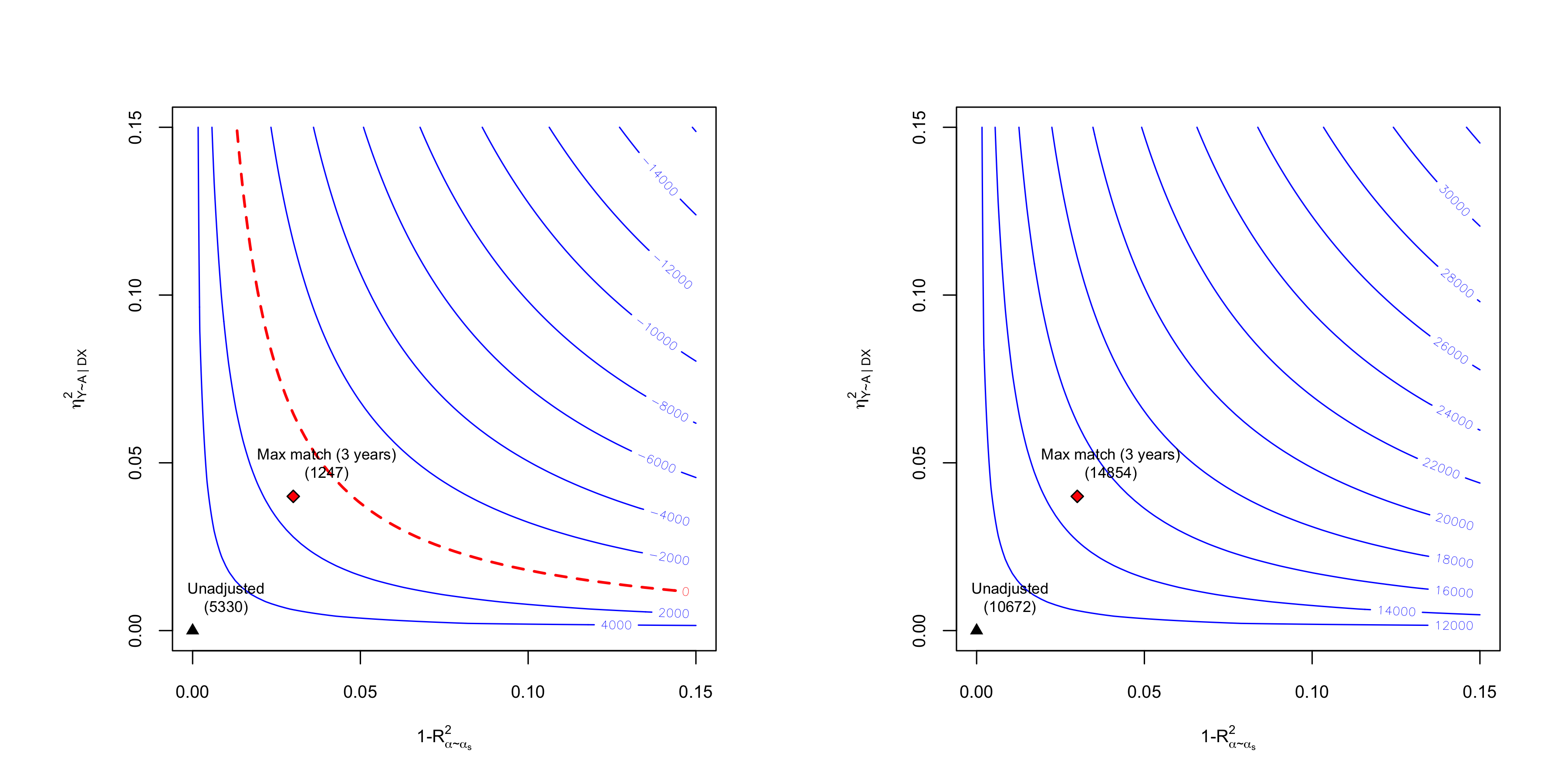
par(oldpar)
# confidence bounds plot
bds   <- confidence_bounds(dml.401k.npm, cf.y = 0.04, cf.d = 0.03, level = 0)
bds   <- setNames(as.data.frame(bds), c("lwr.bound", "upr.bound"))
cbds  <- confidence_bounds(dml.401k.npm, cf.y = 0.04, cf.d = 0.03, level = .95)
cbds  <- setNames(as.data.frame(cbds), c("lwr.cbound", "upr.cbound"))
df2   <- cbind(df, bds[-1,], cbds[-1, ])
ggplot(df2, aes(x = groups, y = estimate)) + geom_line() +
  geom_ribbon(aes(ymin = lwr.bound, ymax = upr.bound),   alpha = 0.1, col = "red", fill = "red") +
  geom_ribbon(aes(ymin = lwr.cbound, ymax = upr.cbound), alpha = 0.1, col = "blue", fill = "blue") +
  theme_bw() +
  xlab("Income Groups by Quartiles") +
  ylab("ATE")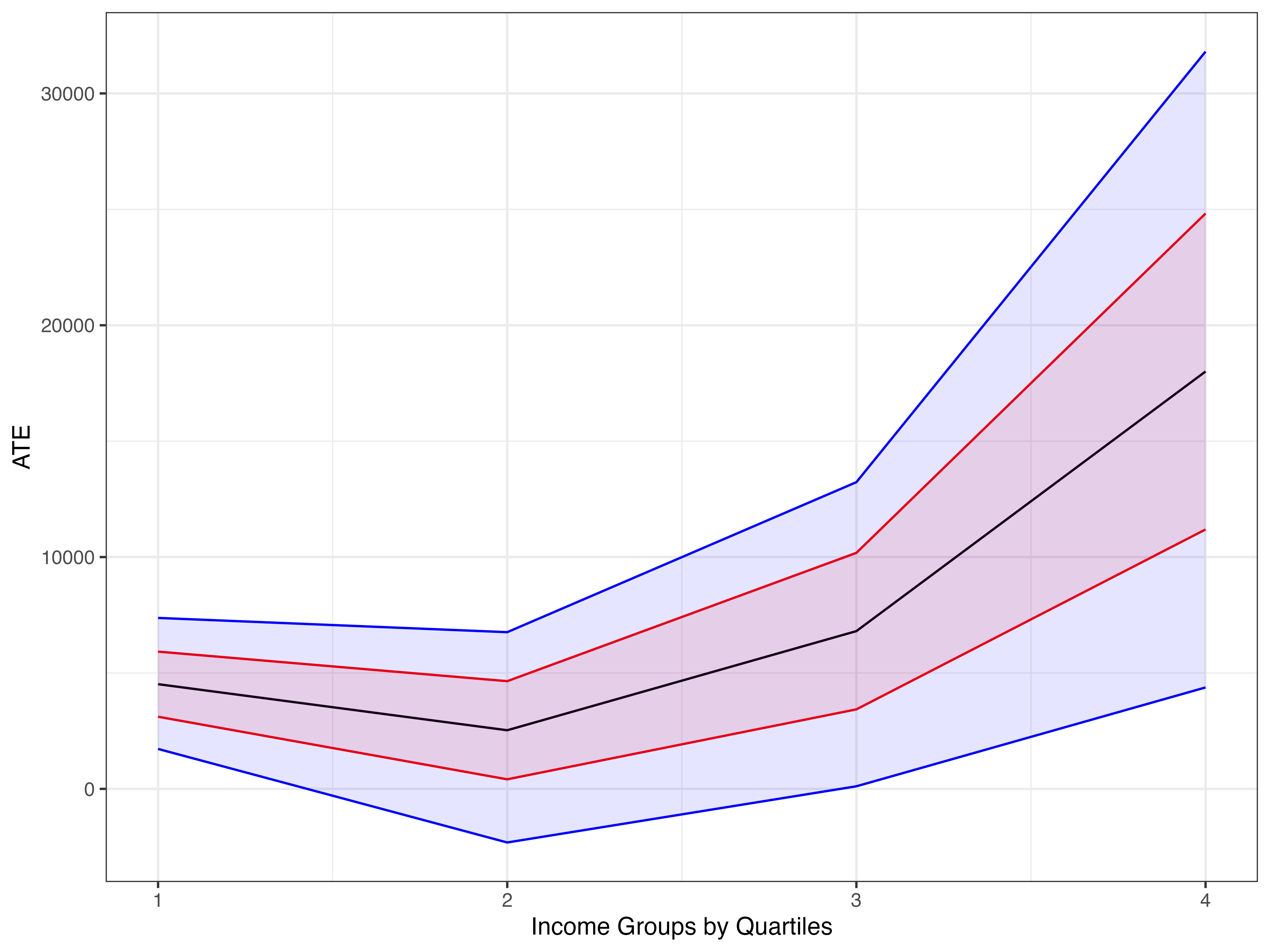
# benchmarks
bench.npm <- dml_benchmark(dml.401k.npm, benchmark_covariates = c("inc", "pira", "twoearn"))
#>
#> === Computing benchmarks using covariate: inc  ===
#>
#> Debiased Machine Learning
#>
#>  Model: Nonparametric
#>  Target: ate
#>  Cross-Fitting: 5 folds, 5 reps
#>  ML Method: outcome (yreg0:ranger, yreg1:ranger), treatment (ranger)
#>  Tuning: dirty
#>
#>
#> ====================================
#> Tuning parameters using all the data
#> ====================================
#>
#> - Tuning Model for D.
#> -- Best Tune:
#>   mtry min.node.size splitrule
#> 1    2             5  variance
#>
#> - Tuning Model for Y (non-parametric).
#> -- Best Tune:
#>   mtry min.node.size splitrule
#> 1    2             5  variance
#>   mtry min.node.size splitrule
#> 1    2             5  variance
#>
#>
#> ======================================
#> Repeating 5-fold cross-fitting 5 times
#> ======================================
#>
#> -- Rep 1 -- Folds: 1  2  3  4  5
#>
#> -- Rep 2 -- Folds: 1  2  3  4  5
#>
#> -- Rep 3 -- Folds: 1  2  3  4  5
#>
#> -- Rep 4 -- Folds: 1  2  3  4  5
#>
#> -- Rep 5 -- Folds: 1  2  3  4  5
#>
#>
#> === Computing benchmarks using covariate: pira  ===
#>
#> Debiased Machine Learning
#>
#>  Model: Nonparametric
#>  Target: ate
#>  Cross-Fitting: 5 folds, 5 reps
#>  ML Method: outcome (yreg0:ranger, yreg1:ranger), treatment (ranger)
#>  Tuning: dirty
#>
#>
#> ====================================
#> Tuning parameters using all the data
#> ====================================
#>
#> - Tuning Model for D.
#> -- Best Tune:
#>   mtry min.node.size splitrule
#> 1    2             5  variance
#>
#> - Tuning Model for Y (non-parametric).
#> -- Best Tune:
#>   mtry min.node.size splitrule
#> 1    2             5  variance
#>   mtry min.node.size splitrule
#> 1    2             5  variance
#>
#>
#> ======================================
#> Repeating 5-fold cross-fitting 5 times
#> ======================================
#>
#> -- Rep 1 -- Folds: 1  2  3  4  5
#>
#> -- Rep 2 -- Folds: 1  2  3  4  5
#>
#> -- Rep 3 -- Folds: 1  2  3  4  5
#>
#> -- Rep 4 -- Folds: 1  2  3  4  5
#>
#> -- Rep 5 -- Folds: 1  2  3  4  5
#>
#>
#> === Computing benchmarks using covariate: twoearn  ===
#>
#> Debiased Machine Learning
#>
#>  Model: Nonparametric
#>  Target: ate
#>  Cross-Fitting: 5 folds, 5 reps
#>  ML Method: outcome (yreg0:ranger, yreg1:ranger), treatment (ranger)
#>  Tuning: dirty
#>
#>
#> ====================================
#> Tuning parameters using all the data
#> ====================================
#>
#> - Tuning Model for D.
#> -- Best Tune:
#>   mtry min.node.size splitrule
#> 1    2             5  variance
#>
#> - Tuning Model for Y (non-parametric).
#> -- Best Tune:
#>   mtry min.node.size splitrule
#> 1    2             5  variance
#>   mtry min.node.size splitrule
#> 1    2             5  variance
#>
#>
#> ======================================
#> Repeating 5-fold cross-fitting 5 times
#> ======================================
#>
#> -- Rep 1 -- Folds: 1  2  3  4  5
#>
#> -- Rep 2 -- Folds: 1  2  3  4  5
#>
#> -- Rep 3 -- Folds: 1  2  3  4  5
#>
#> -- Rep 4 -- Folds: 1  2  3  4  5
#>
#> -- Rep 5 -- Folds: 1  2  3  4  5
bench.npm
#>          gain.Y   gain.D     rho theta.s theta.sj  delta
#> inc     0.13845 0.132481  0.2370    7944    11768 3823.4
#> pira    0.03883 0.006917  0.1160    7944     8448  503.5
#> twoearn 0.01166 0.004419 -0.1459    7944     7469 -475.2