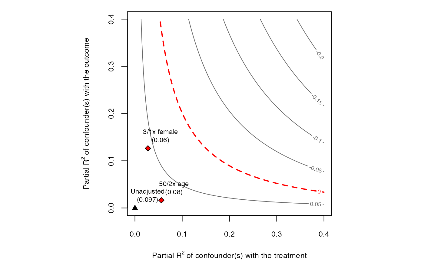
Add bounds to contour plot of omitted variable bias — add_bound_to

Convenience function to add bounds on a sensitivity contour plot created with ovb_contour_plot.

add_bound_to_contour(model, ...)

# S3 method for lm
add_bound_to_contour(
  model,
  benchmark_covariates,
  kd = 1,
  ky = kd,
  bound_label = NULL,
  treatment = plot.env$treatment,
  reduce = plot.env$reduce,
  sensitivity.of = plot.env$sensitivity.of,
  label.text = TRUE,
  cex.label.text = 0.7,
  label.bump.x = plot.env$lim * (1/15),
  label.bump.y = plot.env$lim.y * (1/15),
  round = 2,
  ...
)

# S3 method for fixest
add_bound_to_contour(
  model,
  benchmark_covariates,
  kd = 1,
  ky = kd,
  bound_label = NULL,
  treatment = plot.env$treatment,
  reduce = plot.env$reduce,
  sensitivity.of = plot.env$sensitivity.of,
  label.text = TRUE,
  cex.label.text = 0.7,
  label.bump.x = plot.env$lim * (1/15),
  label.bump.y = plot.env$lim.y * (1/15),
  round = 2,
  ...
)

# S3 method for numeric
add_bound_to_contour(
  r2dz.x,
  r2yz.dx,
  bound_value = NULL,
  bound_label = NULL,
  label.text = TRUE,
  cex.label.text = 0.7,
  font.label.text = 1,
  label.bump.x = plot.env$lim * (1/15),
  label.bump.y = plot.env$lim.y * (1/15),
  round = 2,
  point.pch = 23,
  point.col = "black",
  point.bg = "red",
  point.cex = 1,
  point.font = 1,
  ...
)

Arguments

model: An fixest object with the outcome regression.
...: arguments passed to other methods.
benchmark_covariates: The user has two options: (i) character vector of the names of covariates that will be used to bound the plausible strength of the unobserved confounders. Each variable will be considered separately; (ii) a named list with character vector names of covariates that will be used, as a group, to bound the plausible strength of the unobserved confounders. The names of the list will be used for the benchmark labels. Note: for factor variables with more than two levels, you need to provide the name of each level as encoded in the fixest model (the columns of model.matrix).
kd: numeric vector. Parameterizes how many times stronger the confounder is related to the treatment in comparison to the observed benchmark covariate. Default value is 1 (confounder is as strong as benchmark covariate).
ky: numeric vector. Parameterizes how many times stronger the confounder is related to the outcome in comparison to the observed benchmark covariate. Default value is the same as kd.
bound_label: label to bounds provided manually in r2dz.x and r2yz.dx.
treatment: A character vector with the name of the treatment variable of the model.
reduce: Should the bias adjustment reduce or increase the absolute value of the estimated coefficient? Default is TRUE.
sensitivity.of: should the contour plot show adjusted estimates ("estimate") or adjusted t-values ("t-value")?
label.text: should label texts be plotted? Default is TRUE.
cex.label.text: size of the label text.
label.bump.x: bump on the x coordinate of label text.
label.bump.y: bump on the y coordinate of label text.
round: integer indicating the number of decimal places to be used for rounding.
r2dz.x: Hypothetical partial R2 of unobserved confounder Z with treatment D, given covariates X.
r2yz.dx: Hypothetical partial R2 of unobserved confounder Z with outcome Y, given covariates X and treatment D.
bound_value: value to be printed in label bound.
font.label.text: font for the label text.
point.pch: plotting character for points.
point.col: color code or name for points.
point.bg: backgrounf (fill) color for points.
point.cex: size of points.
point.font: font for points.

Value

The function adds bounds in an existing contour plot and returns `NULL`.

Examples


# runs regression model
model <- lm(peacefactor ~ directlyharmed + age + farmer_dar + herder_dar +
                         pastvoted + hhsize_darfur + female + village,
                         data = darfur)
# contour plot
ovb_contour_plot(model = model, treatment = "directlyharmed")

# add bound 3/1 times stronger than female
add_bound_to_contour(model = model,
                     benchmark_covariates = "female",
                     kd = 3, ky = 1)

# add bound 50/2 times stronger than age
add_bound_to_contour(model = model,
                     benchmark_covariates = "age",
                     kd = 50, ky = 2)