Sensitivity Analysis of Instrumental Variable Estimates

This function performs sensitivity analysis of instrumental variable estimates, as discussed in Cinelli and Hazlett (2025). The main input is an object of class iv_fit. It returns an object of class iv.sensemakr with several pre-computed sensitivity statistics for reporting. After running sensemakr you may directly use the plot, print and summary methods in the returned object.

Usage

sensemakr(...)

# S3 method for class 'iv_fit'
sensemakr(
  model,
  benchmark_covariates = NULL,
  kz = 1,
  ky = kz,
  kd = kz,
  r2zw.x = NULL,
  r2y0w.zx = r2zw.x,
  bound_label = "Manual Bound",
  q = 1,
  alpha = 0.05,
  min = TRUE,
  ...
)

Arguments

...: arguments passed to other methods.
model: a model created with the function iv_fit.
benchmark_covariates: character vector of the names of covariates that will be used to bound the plausible strength of the latent variables.
kz: numeric vector. Parameterizes how many times stronger the latent variables are related to the instrument in comparison to the observed benchmark covariates. Default value is 1 (latent variable is as strong as benchmark covariate).
ky: numeric vector. Parameterizes how many times stronger the latent variables are related to the (pot.) outcome in comparison to the observed benchmark covariates.
kd: numeric vector. Parameterizes how many times stronger the latent variables are related to the treatment in comparison to the observed benchmark covariates. Default value is the same as kz.
r2zw.x: (optional) hypothetical partial R2 of latent variables W with the instrument Z, given observed covariates X.
r2y0w.zx: (optional) hypothetical partial R2 of latent variables W with the (pot.) outcome Y(0) given Z and X. Default is the same as r2zw.x.
bound_label: label to bounds provided manually in r2zw.x and r2y0w.zx.
q: percent change of the effect estimate that would be deemed problematic. Default is 1, which means a reduction of 100% of the current effect estimate (bring estimate to zero).
alpha: significance level.
min: should we consider biases as large or larger than a certain amount? Default is TRUE.

Value

An object of class iv.sensemakr, containing:

pars: A list with the general parameters used when calling sensemakr.
unadjusted: A list with the original, unadjusted results.
sensitivity_stats: A list with the sensitivity statistics of the IV, First-Stage, and Reduced-Form regressions.
bounds: A list with bounds on the strength of latent variables if they were "k times" as strong as the benchmark covariates.

References

Cinelli, C. and Hazlett, C. (2025), "An Omitted Variable Bias Framework for Sensitivity Analysis of Instrumental Variables." Biometrika. doi:10.1093/biomet/asaf004

Examples


# loads package
library(iv.sensemakr)

# loads dataset
data("card")

# prepares data
y <- card$lwage  # outcome
d <- card$educ   # treatment
z <- card$nearc4 # instrument
x <- model.matrix( ~ exper + expersq + black + south + smsa + reg661 + reg662 +
                     reg663 + reg664 + reg665+ reg666 + reg667 + reg668 + smsa66,
                   data = card) # covariates
# fits IV model
card.fit <- iv_fit(y,d,z,x)

# see results
card.fit
#> 
#> Instrumental Variable Estimation
#> (Anderson-Rubin Approach)
#> =============================================
#> IV Estimates:
#>   Coef. Estimate: 0.132
#>   t-value: 2.33
#>   p-value: 0.02
#>   Conf. Interval: [0.025, 0.285]
#> Note: H0 = 0, alpha = 0.05, df = 2994.
#> =============================================
#> See summary for first stage and reduced form.
#> 

# runs sensitivity analysis
card.sens <- sensemakr(card.fit, benchmark_covariates = c("black", "smsa"))

# see results
card.sens
#> 
#> Sensitivity Analysis for Instrumental Variables
#> (Anderson-Rubin Approach)
#> =============================================================
#> IV Estimates:
#>   Coef. Estimate: 0.132
#>   t-value: 2.33
#>   p-value: 0.02
#>   Conf. Interval: [0.025, 0.285]
#> 
#> Sensitivity Statistics:
#>   Extreme Robustness Value: 0.000523
#>   Robustness Value: 0.00667
#> 
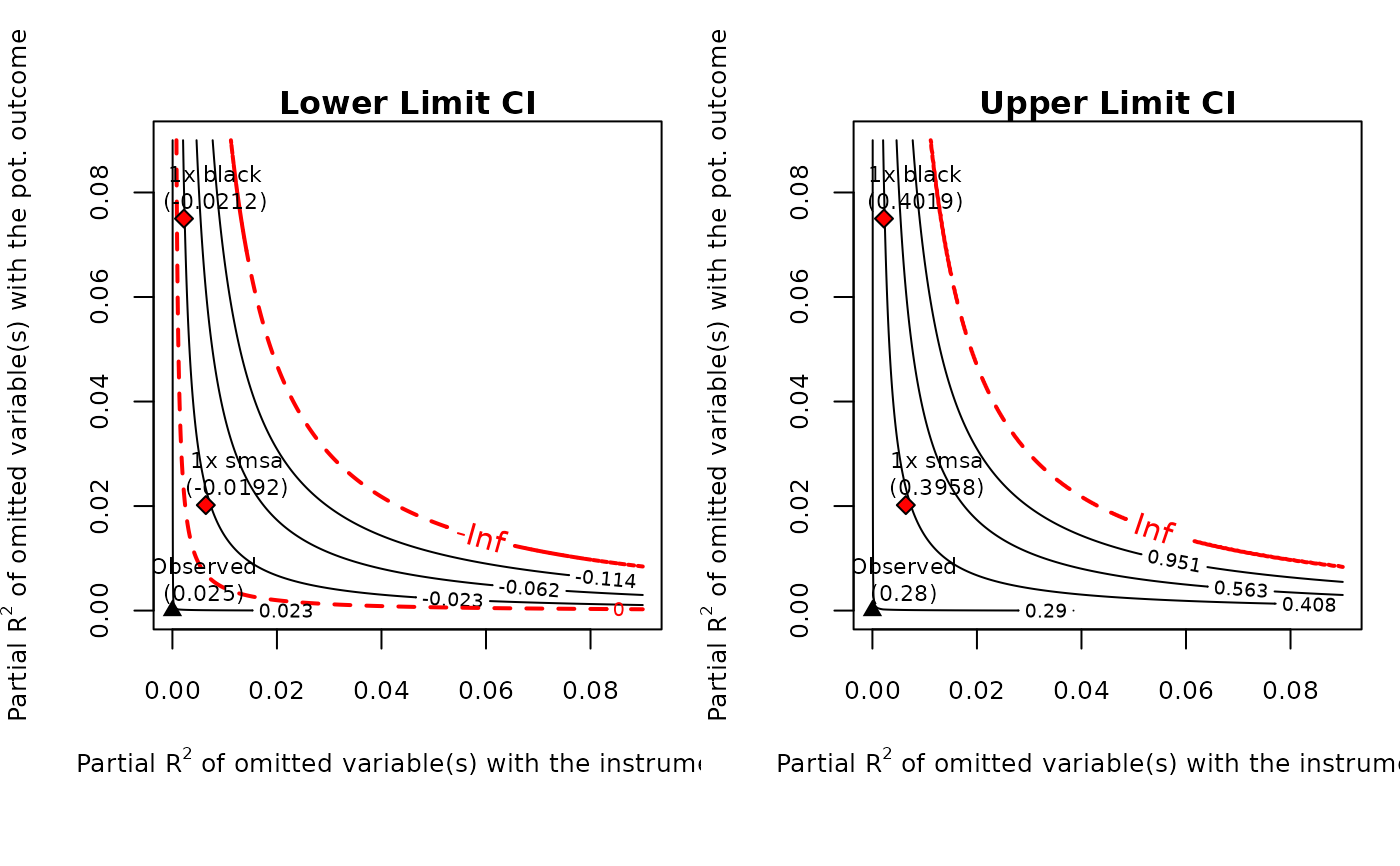
#> Bounds on Omitted Variable Bias:
#>  Bound Label  R2zw.x R2y0w.zx Lower CI Upper CI Crit. Thr.
#>     1x black 0.00221   0.0750  -0.0212    0.402       2.59
#>      1x smsa 0.00639   0.0202  -0.0192    0.396       2.57
#> 
#> Note: H0 = 0, q >= 1, alpha = 0.05, df = 2994.
#> =============================================================
#> See summary for first stage and reduced form.
#> 

# sensitivity contour plot
plot(card.sens, lim = 0.09)