iv.sensemakr implements a suite of sensitivity analysis tools for instrumental variable estimates, as discussed in Cinelli, C. and Hazlett, C. (2025) “An Omitted Variable Bias Framework for Sensitivity Analysis of Instrumental Variables”, Biometrika (doi:10.1093/biomet/asaf004; PDF).
News
iv.sensemakris now on CRAN!Package website is now online.
Paper published in Biometrika. You can find a free version here..
Watch the video of the talk at PCIC.
Watch the video of the talk at JSM.
Installation
To install iv.sensemakr from CRAN:
install.packages("iv.sensemakr")To install the development version from GitHub, make sure you have the package devtools installed:
# install.packages("devtools")
devtools::install_github("carloscinelli/iv.sensemakr")
Basic usage
# loads package
library(iv.sensemakr)

# loads dataset
data("card")

# prepares data
y <- card$lwage  # outcome
d <- card$educ   # treatment
z <- card$nearc4 # instrument
x <- model.matrix( ~ exper + expersq + black + south + smsa + reg661 + reg662 +
                     reg663 + reg664 + reg665+ reg666 + reg667 + reg668 + smsa66,
                   data = card) # covariates
# fits IV model
card.fit <- iv_fit(y,d,z,x)

# see results
card.fit
#>
#> Instrumental Variable Estimation
#> (Anderson-Rubin Approach)
#> =============================================
#> IV Estimates:
#>   Coef. Estimate: 0.132
#>   t-value: 2.33
#>   p-value: 0.02
#>   Conf. Interval: [0.025, 0.285]
#> Note: H0 = 0, alpha = 0.05, df = 2994.
#> =============================================
#> See summary for first stage and reduced form.

# runs sensitivity analysis
card.sens <- sensemakr(card.fit, benchmark_covariates = c("black", "smsa"))

# see results
card.sens
#>
#> Sensitivity Analysis for Instrumental Variables
#> (Anderson-Rubin Approach)
#> =============================================================
#> IV Estimates:
#>   Coef. Estimate: 0.132
#>   t-value: 2.33
#>   p-value: 0.02
#>   Conf. Interval: [0.025, 0.285]
#>
#> Sensitivity Statistics:
#>   Extreme Robustness Value: 0.000523
#>   Robustness Value: 0.00667
#>
#> Bounds on Omitted Variable Bias:
#>  Bound Label  R2zw.x R2y0w.zx Lower CI Upper CI Crit. Thr.
#>     1x black 0.00221   0.0750  -0.0212    0.402       2.59
#>      1x smsa 0.00639   0.0202  -0.0192    0.396       2.57
#>
#> Note: H0 = 0, q >= 1, alpha = 0.05, df = 2994.
#> =============================================================
#> See summary for first stage and reduced form.

# sensitivity contour plot
plot(card.sens, lim = 0.09)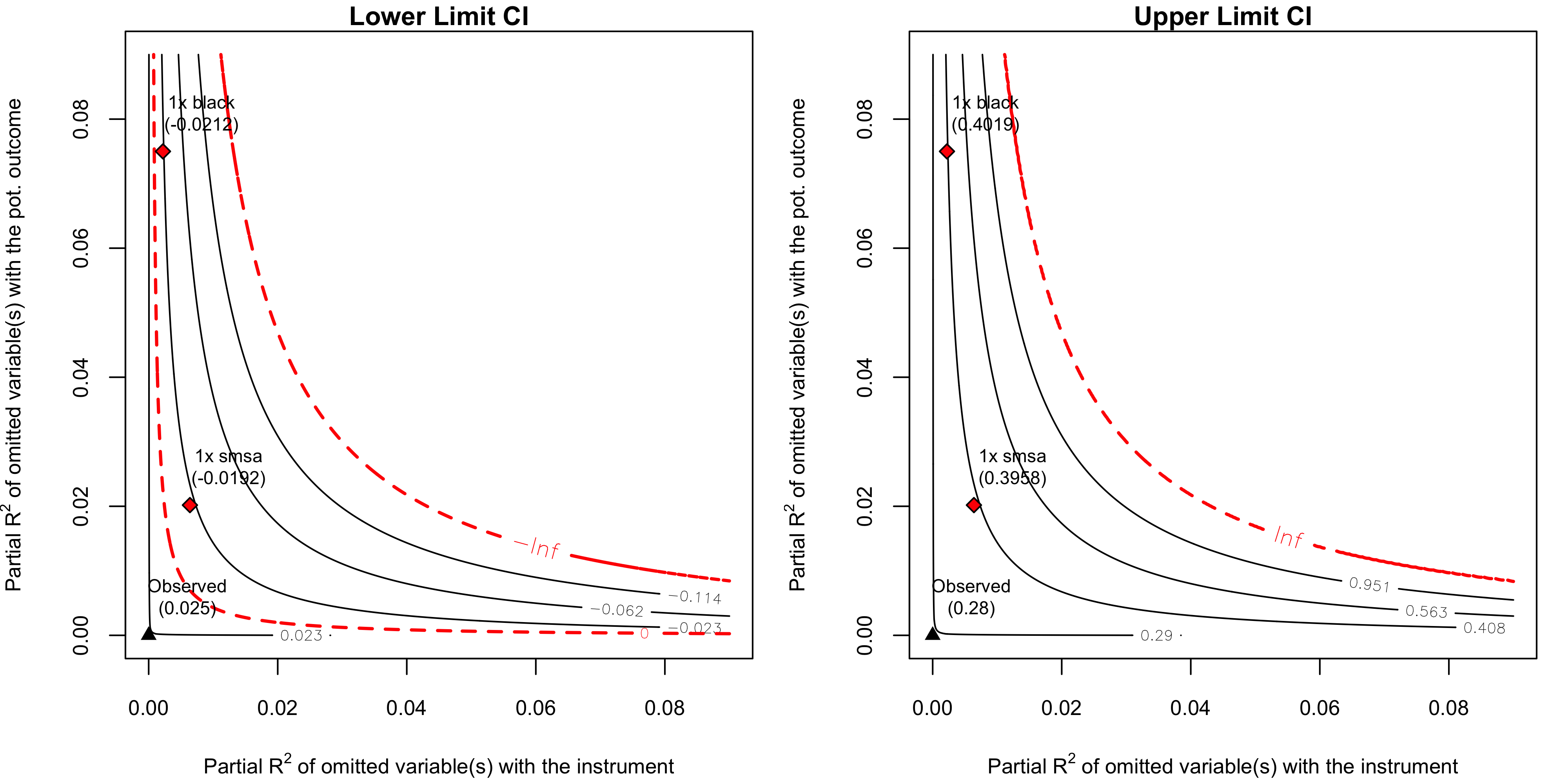
# latex code for sensitivity table
ovb_minimal_reporting(card.sens, outcome_label = "lwage", treatment_label = "educ")
#> \begin{table}[!h]
#> \centering
#> \begin{tabular}{lrrrrrr}
#> \multicolumn{7}{c}{Outcome: \textit{lwage}} \\
#> \hline \hline
#> Treatment: & Est. & Lower CI & Upper CI & t-value & $XRV_{q = 1, \alpha = 0.05}$ & $RV_{q = 1, \alpha = 0.05}$  \\
#> \hline
#> \textit{educ} & 0.132 & 0.025 & 0.285 & 2.327 & 0.1\% & 0.7\% \\
#> \hline
#> df = 2994 & & \multicolumn{5}{r}{ \small \textit{Bound (1x black)}: $R^2_{Z\sim W| {\bf X}}$ = 0.2\%, $R^2_{Y(0)\sim W| Z, {\bf X}}$ = 7.5\%} \\
#> \end{tabular}
#> \end{table}
# html code for sensitivity table
ovb_minimal_reporting(card.sens, format = "pure_html",
outcome_label = "lwage", treatment_label = "educ")| Outcome: lwage | ||||||
|---|---|---|---|---|---|---|
| Treatment | Est. | Lower CI | Upper CI | t-value | XRVq = 1, α = 0.05 | RVq = 1, α = 0.05 |
| educ | 0.132 | 0.025 | 0.285 | 2.327 | 0.1% | 0.7% |
| Note: df = 2994; Bound ( 1x black ): R2Z~W|X = 0.2%, R2Y(0)~W|Z,X = 7.5% | ||||||