Sensitivity Analysis for Instrumental Variables using `iv.sensemakr`

Introduction

Instrumental variable (IV) methods are widely used in economics, epidemiology, and the social sciences to estimate causal effects in the presence of unobserved confounding. A valid IV approach requires that, conditionally on observed covariates, the instrument is not itself confounded with the outcome, and that it influences the outcome only by affecting uptake of the treatment. The first assumption is usually called “exogeneity,” “ignorability,” or “unconfoundedness” of the instrument, whereas the second is usually called the “exclusion restriction.”

However, these assumptions are often violated in practice due to the presence of omitted confounders of the instrument; or, even when the instrument is randomized, by omitted side-effects of the instrument influencing the outcome via paths other than through the treatment. If these assumptions fail, the bias of the IV estimate may in fact be worse than the original confounding bias of the naive regression estimate. Researchers are therefore often advised to perform sensitivity analyses to assess the degree of violation of the IV assumptions required to alter the conclusions of an IV study.

The package iv.sensemakr aims to help with this task, implementing a suite of sensitivity analysis tools for IV estimates as developed in Cinelli and Hazlett (2025), which builds on the omitted variable bias (OVB) framework of Cinelli and Hazlett (2020). The goal of iv.sensemakr is to make it easier to understand how violations of unconfoundedness of the instrument or the exclusion restriction would affect the original findings of a study.

Estimating the returns to schooling

Since sensitivity analysis requires contextual knowledge to be properly interpreted, we illustrate the basic functionality of the package with a real example. Here we reproduce the results found in Section 5 of Cinelli and Hazlett (2025). Card (1993) used proximity to college as an instrumental variable to estimate the causal effect of education on earnings. We revisit that study and quantify how robust the initial findings are to violations of the IV assumptions.

The data

The card dataset is included in the package, and consists of a sample of $n = 3{,}010$ individuals from the National Longitudinal Survey of Young Men. The key variables are:

lwage: log hourly wage in 1976 (outcome).
educ: years of completed education (treatment).
nearc4: indicator for proximity to a four-year college (instrument).

There are also various covariates, such as experience (exper), experience squared (expersq), race (black), whether the individual lived in a standard metropolitan area (smsa), and geographic region dummies. One can load the dataset with the following command.

# load the package
library(iv.sensemakr)

# load the dataset
data("card")

OLS findings and the OVB problem

In a regression of log wages ( $Y$ ) on years of education ( $D$ ), adjusting for race, experience, and regional factors ( $X$ ), Card found that each additional year of schooling was associated with approximately 7.5% higher wages. We can reproduce this finding with a simple OLS regression.

# OLS regression of log wages on education and covariates
card.ols <- lm(lwage ~ educ + exper + expersq + black + south + smsa + reg661 +
                  reg662 + reg663 + reg664 + reg665 + reg666 +
                  reg667 + reg668 + smsa66,
                data = card)
coef(card.ols)["educ"]
#>       educ 
#> 0.07469326
confint(card.ols)["educ", ]
#>      2.5 %     97.5 % 
#> 0.06783385 0.08155266

However, educational achievement is not randomly assigned. Individuals who obtain more education may have higher wages for other reasons, such as family background, regional differences, or higher levels of some unobserved characteristic such as ability or motivation. Regression estimates such as the above, that adjust for only a partial list of characteristics, may thus suffer from omitted variable bias, likely overestimating the true returns to schooling. This motivates the use of instrumental variables.

Original IV estimates

IV methods offer an alternative route to estimating the causal effect of schooling on earnings without having data on those unobserved variables. The key is to find a new variable—the instrument, here denoted by $Z$ —that changes the incentives to educational achievement, but is associated with earnings only through its effect on education. Card proposed exploiting the role of geographic differences in college accessibility as an instrumental variable. The instrument nearc4 encodes whether the individual grew up near a four-year college. Students who grow up far from college may face higher educational costs, discouraging them from pursuing higher-level studies. More importantly, Card argues that whether one lives near a college is not itself confounded with earnings, nor does it cause earnings apart from its effect on years of education.

Given these two assumptions, one can use nearc4 as an IV for the effect of educ on lwage. Such estimates can be obtained using the iv_fit() function, which takes as input vectors for the outcome y, treatment d, instrument z, and an optional covariate matrix x. It computes IV estimates using the Anderson-Rubin (AR) approach (Anderson and Rubin, 1949), which is numerically equivalent to Two-Stage Least Squares (2SLS) for point estimation, but constructs confidence intervals via test inversion, a procedure that has correct coverage regardless of instrument strength.

# prepare data
y <- card$lwage  # outcome: log wage
d <- card$educ   # treatment: years of education
z <- card$nearc4 # instrument: proximity to college
x <- model.matrix(~ exper + expersq + black + south + smsa + reg661 +
                     reg662 + reg663 + reg664 + reg665 + reg666 +
                     reg667 + reg668 + smsa66,
                   data = card)

# fit the IV model
card.fit <- iv_fit(y, d, z, x)
card.fit
#> 
#> Instrumental Variable Estimation
#> (Anderson-Rubin Approach)
#> =============================================
#> IV Estimates:
#>   Coef. Estimate: 0.132
#>   t-value: 2.33
#>   p-value: 0.02
#>   Conf. Interval: [0.025, 0.285]
#> Note: H0 = 0, alpha = 0.05, df = 2994.
#> =============================================
#> See summary for first stage and reduced form.

The IV estimate suggests that each additional year of schooling raises wages by about 13.2%, which is not only positive but, perhaps surprisingly, much higher than the simple OLS estimate of 7.5%. But how much can we trust the IV estimate? Is proximity to college really a valid instrument?

The IV estimate may suffer from omitted variable bias

The previous IV estimate relies on the assumption that, conditional on $X$ , proximity to college and earnings are unconfounded, and that the effect of proximity on earnings goes entirely through education. As is often the case, neither assumption is easy to defend. The same factors that might confound the relationship between education and earnings could similarly confound the relationship between proximity to college and earnings (e.g., family wealth or connections). Moreover, the presence of a college nearby may be associated with high school quality, which in turn also affects earnings. Finally, geographic factors can make some localities likely to both have colleges nearby and lead to higher earnings—these are only coarsely conditioned on by the observed regional indicators, and residual biases may remain.

Therefore, instead of adjusting for $X$ only, we should have adjusted for both the observed covariates $X$ and unobserved covariates $W$ , where $W$ stands for all unobserved factors necessary to make proximity to college a valid instrument for the effect of education on earnings. How do the IV estimates from the model omitting $W$ compare with the estimates we actually want, from the model that includes $W$ ?

Sensitivity analysis

The main function of the package is sensemakr(). It takes an iv_fit object as input and performs the most commonly required sensitivity analyses, which can then be further explored with the print, summary, and plot methods. We begin by applying sensemakr to the card.fit object.

# with all parameters shown explicitly
card.sens <- sensemakr(model = card.fit,
                       benchmark_covariates = c("black", "smsa"),
                       kz = 1,               # benchmark multiplier for Z
                       ky = 1,               # benchmark multiplier for Y
                       q = 1,                # reduce estimate to zero
                       alpha = 0.05)         # significance level

The arguments of the call are:

model: the iv_fit object with the original IV regression.
benchmark_covariates: the names of observed covariates that will be used to bound the plausible strength of the omitted variables. Here we use "black" (an indicator of race) and "smsa" (an indicator of whether the individual lived in a standard metropolitan area).
kz, ky: these arguments parameterize how many times stronger omitted variables are related to the instrument (kz) and to the untreated potential outcome (ky) in comparison to the observed benchmark covariates. For example, setting kz=1 and ky=1 means that we will consider unobserved confounders or side-effects as strong as "black" or "smsa".
q: the fraction of the effect estimate that would have to be explained away to be deemed problematic. Setting q = 1, as we do here, means that a reduction of 100% of the current effect estimate—that is, a true effect of zero—would be problematic. The default is 1.
alpha: significance level of interest for statistical inference. The default is 0.05.

Using the default arguments, one can simplify the previous call to:

card.sens <- sensemakr(card.fit, benchmark_covariates = c("black", "smsa"))

Minimal sensitivity reporting

The print method of sensemakr provides a quick review of the original estimate along with two summary sensitivity statistics suited for routine reporting.

card.sens
#> 
#> Sensitivity Analysis for Instrumental Variables
#> (Anderson-Rubin Approach)
#> =============================================================
#> IV Estimates:
#>   Coef. Estimate: 0.132
#>   t-value: 2.33
#>   p-value: 0.02
#>   Conf. Interval: [0.025, 0.285]
#> 
#> Sensitivity Statistics:
#>   Extreme Robustness Value: 0.000523
#>   Robustness Value: 0.00667
#> 
#> Bounds on Omitted Variable Bias:
#>  Bound Label  R2zw.x R2y0w.zx Lower CI Upper CI Crit. Thr.
#>     1x black 0.00221   0.0750  -0.0212    0.402       2.59
#>      1x smsa 0.00639   0.0202  -0.0192    0.396       2.57
#> 
#> Note: H0 = 0, q >= 1, alpha = 0.05, df = 2994.
#> =============================================================
#> See summary for first stage and reduced form.

The robustness value (RV) describes the minimum partial $R^2$ that confounders or side-effects would need to have with both the instrument and the untreated potential outcome in order to make the adjusted confidence interval include zero. In the Card example, the RV is about 0.67%, revealing that confounders or side-effects explaining 0.67% of the residual variation of both the instrument and the potential outcome are already sufficiently strong to make the IV estimate statistically insignificant. On the other hand, confounders that do not explain at least 0.67% of the residual variation of both the instrument and the potential outcome are not sufficiently strong to do so.

The extreme robustness value (XRV) describes the minimum strength of association that omitted variables need to have with the instrument alone in order to be problematic. The XRV of 0.05% means that, if we are not willing to impose constraints on the partial $R^2$ of omitted variables with the outcome, then such omitted variables need only explain 0.05% of the residual variation of the instrument to be problematic. This is a worst-case measure: it considers the scenario in which confounders may explain an arbitrarily large share of the outcome’s residual variation, and asks how much of the instrument’s variation they would still need to explain.

These are useful quantities that summarize what we need to know in order to safely rule out confounders or side-effects that are deemed problematic. Interpreting these values requires domain knowledge about the data-generating process. Are values of 0.67% or 0.05% enough to be confident in the original findings? One way to assess the plausibility of omitted variables with such strength is to consider confounders or side-effects as strong as observed covariates. This is given by the table named “Bounds on Omitted Variable Bias,” which shows how strong omitted variables would be if they were as strong as black or smsa. As we can see, such variables would be sufficiently strong to overturn the results of the original study. Since it is not very difficult to imagine residual confounding as strong or stronger than those variables (e.g., parental income, finer-grained geographic location, etc), these results are already sufficient to call into question the strength of evidence provided by this study.

Sensitivity contour plots

The previous sensitivity table provides a good summary of how robust the current estimate is to confounding. However, researchers may wish to refine their analysis by visually exploring the full range of possible estimates that omitted variables of different strengths could produce. For this, one can use the plot method for sensemakr.

plot(card.sens, lim = 0.09)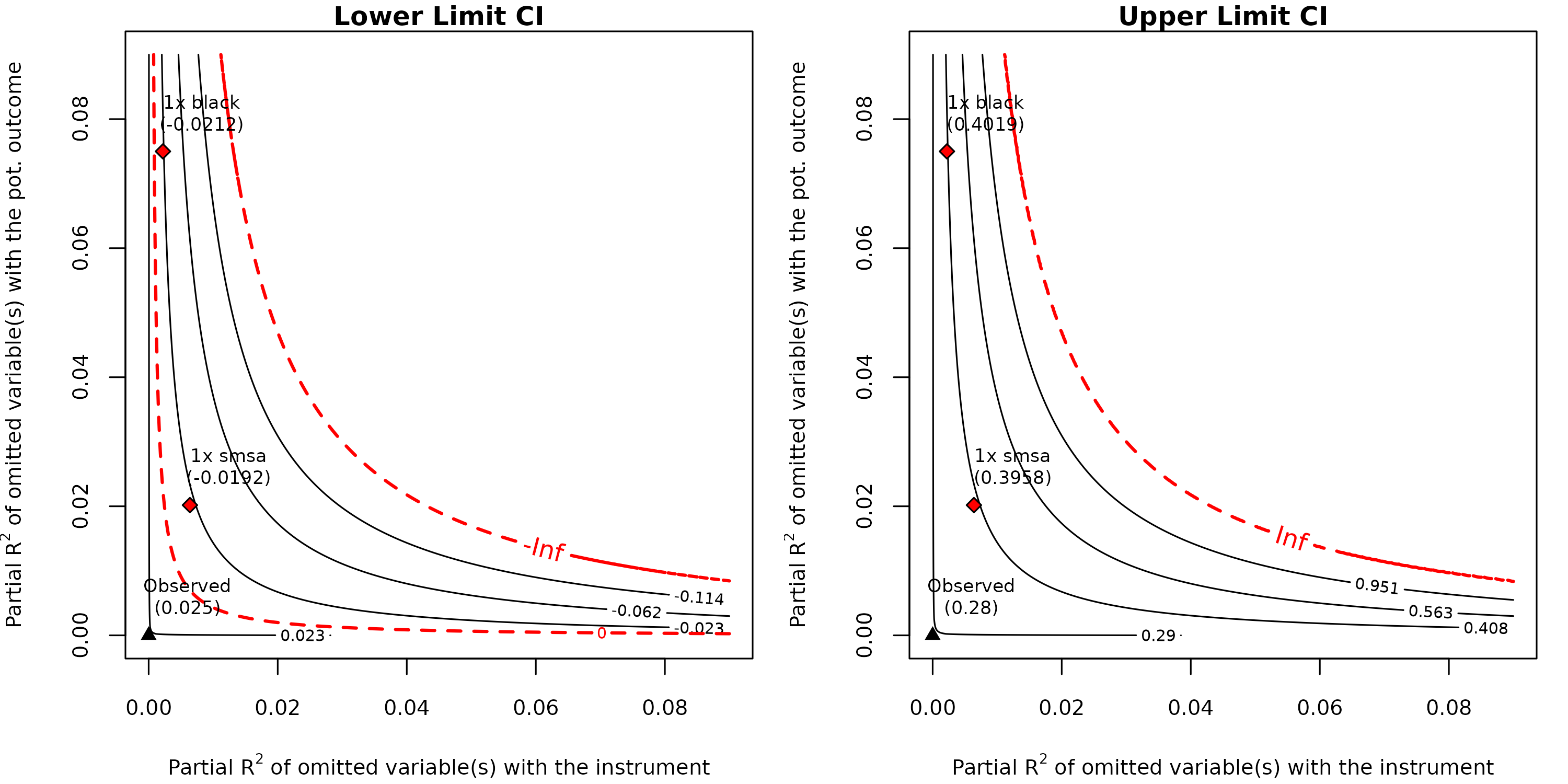

The left plot shows bounds on the lower limit of the confidence interval, whereas the right plot shows bounds on the upper limit. In both cases, the horizontal axis shows the hypothetical partial $R^2$ of omitted variables with the instrument, and the vertical axis shows the hypothetical partial $R^2$ of omitted variables with the untreated potential outcome. The contour lines show what the lower or upper limit of the confidence interval would be, had we adjusted for omitted variables with such hypothetical strengths. The point labeled “Observed” at the origin represents the original IV estimate, which assumes no violation of the IV assumptions. As we move away from the origin—that is, as the hypothetical omitted variables become stronger—the confidence interval widens. The red dashed line marks both the critical threshold (zero), as well as the boundary beyond which the confidence intervals become unbounded. The labeled points show the benchmark bounds for the observed covariates black and smsa, indicating where confounders of comparable strength would fall on this plot. Note that any other scenario can also be contemplated here, by simply picking different pairs of $R^2$ values. As we had seen in our previous analysis, confounding as strong as "smsa" or "black" could lead to an interval of [-0.02, 0.40], which includes not only implausibly high values (40%) but also negative values (-2%) showing that the IV estimate is very fragile to any residual confounding of such magnitudes.

References

Anderson, T.W. and Rubin, H. (1949), “Estimation of the parameters of a single equation in a complete system of stochastic equations.” Annals of Mathematical Statistics, 20, 46–63.

Card, D. (1993). Using geographic variation in college proximity to estimate the return to schooling. Technical report, National Bureau of Economic Research.

Cinelli, C. and Hazlett, C. (2020), “Making sense of sensitivity: Extending omitted variable bias.” Journal of the Royal Statistical Society, Series B (Statistical Methodology), 82(1), 39–67. doi:10.1111/rssb.12348.

Cinelli, C. and Hazlett, C. (2025), “An omitted variable bias framework for sensitivity analysis of instrumental variables.” Biometrika, 112(1). doi:10.1093/biomet/asaf004.

Carlos Cinelli and Chad Hazlett

2026-02-09