The Risks of Informal Benchmarking • sensemakr

Introduction

Informal “benchmarking” procedures have been widely suggested in the sensitivity analysis literature as a means to aid interpretation. It intends to describe how an unobserved confounder \(Z\) “not unlike” some observed covariate \(X_j\) would alter the results of a study (e.g., Imbens, 2003; Blackwell, 2013; Hosman et al. 2010, Dorie et al., 2016, Hong et al. 2018). Cinelli and Hazlett (2020) show why these proposals may lead users to erroneous conclusions, and offer formal bounds on the bias that could be produced by unobserved confounding “as strong” as certain observed covariates.

To aid in understanding and appreciating the risk of informal benchmarking procedures, this vignette replicates the example in Section 6.1 of Cinelli and Hazlett (2020), in which such benchmarks produce clearly misleading results. Replicating this example with sensemakr also provides a useful tutorial on how users can construct their own sensitivity contour plots with customized bounds, beyond what is offered by default on the package.

Background

Prior work in sensitivity analysis—dating back at least to Imbens (2003), and followed by others (e.g, Hosman et al. 2010, Dorie et al., 2016, Hong et al. 2018)—has proposed comparing observables with unobservables by informally using statistics of observed variables to “calibrate intuitions” about sensitivity parameters concerning the unobserved variable. This practice, however, can have undesirable consequences, illustrated below. Section 4.4 of Cinelli and Hazlett (2020) provides an alternative. This approach bounds the maximum strength of confounding given relative judgments on how the strength unobserved variables compares to the strength of observed variables. The sensemakr package allows us to compute such bounds using the function ovb_bounds(), which we demonstrate below.

Simulating the data

Let us begin by simulating the data generating process used in our example. Consider a treatment variable \(D\), an outcome variable \(Y\), one observed confounder \(X\), and one unobserved confounder \(Z\). Again, all disturbance variables \(U\) are standardized mutually independent gaussians, and note that, in reality, the treatment \(D\) has no causal effect on the outcome \(Y\).

\[\begin{align} Z &= U_{z}\\ X &= U_{x}\\ D &= X + Z + U_d\\ Y &= X + Z + U_y \end{align}\]

Also note that, in this model: (i) the unobserved confounder \(Z\) is independent of \(X\); and, (ii) the unobserved confounder \(Z\) is exactly like \(X\) in terms of its strength of association with the treatment and the outcome. The code below creates a sample of size 100 of this data generating process. We make sure to create residuals that are standardized and orthogonal so that all properties that we describe here will hold exactly even in this finite sample.

# loads sensemakr package
library(sensemakr)
#> See details in:
#> Carlos Cinelli and Chad Hazlett (2020). Making Sense of Sensitivity: Extending Omitted Variable Bias. Journal of the Royal Statistical Society, Series B (Statistical Methodology).

# simulates data
n <- 100
X <- scale(rnorm(n))
Z <- resid_maker(n, X) 
D <- X + Z + resid_maker(n, cbind(X, Z)) 
Y <- X + Z + resid_maker(n, cbind(X, Z, D))

Fitting the model

In this example, the investigator does not observe the confounder \(Z\). Therefore, she is forced to fit the restricted linear model \(Y \sim D + X\), resulting in the following estimated values

model.ydx <- lm(Y ~ D + X) 
summary(model.ydx)
#> 
#> Call:
#> lm(formula = Y ~ D + X)
#> 
#> Residuals:
#>     Min      1Q  Median      3Q     Max 
#> -3.4250 -0.8597  0.1516  0.8094  2.7530 
#> 
#> Coefficients:
#>              Estimate Std. Error t value Pr(>|t|)    
#> (Intercept) 7.772e-17  1.237e-01   0.000  1.00000    
#> D           5.000e-01  8.793e-02   5.686 1.37e-07 ***
#> X           5.000e-01  1.523e-01   3.283  0.00143 ** 
#> ---
#> Signif. codes:  0 '***' 0.001 '**' 0.01 '*' 0.05 '.' 0.1 ' ' 1
#> 
#> Residual standard error: 1.237 on 97 degrees of freedom
#> Multiple R-squared:    0.5,  Adjusted R-squared:  0.4897 
#> F-statistic:  48.5 on 2 and 97 DF,  p-value: 2.512e-15

Note we obtain a large and statistically significant coefficient estimate of the effect of \(X\) on \(Y\) (\(0.5\)). However, we know that the variable \(Z\) is not observed, and there is the fear that this estimated effect is in fact due to the bias caused by \(Z\). On the other hand, let us suppose the investigator correctly knows that: (i) \(Z\) and \(X\) have the same strength of association with \(D\) and \(Y\); and, (ii) \(Z\) is independent of \(X\). Can we leverage this information to understand how much bias a confounder \(Z\) “not unlike” \(X\) could cause?

Informal benchmarks

Computing the bias due to the omission of \(Z\) requires two sensitivity parameters: its partial \(R^2\) with the treatment \(D\) and its partial \(R^2\) with the outcome \(Y\). How could we go about computing the bias that a confounder \(Z\) “not unlike \(X\)” would cause?

Intuitively, it seems that we could take as reference the observed partial \(R^2\) of \(X\) with \(D\) and \(Y\), and use those as the plausible values for the sensitivity parameters. That’s the essence of many informal benchmarking proposals. So let us now compute those observed partial \(R^2\) using the partial_r2() function of sensemakr. For the partial \(R^2\) of \(X\) with the treatment, we also need to fit a treatment regression \(D \sim X\) first.

# fits treatment regression
model.dx <- lm(D ~ X)

# computes observed partial R2 of X
r2yx.d <- partial_r2(model.ydx, covariates = "X")
r2dx   <- partial_r2(model.dx, covariates = "X")

Once both partial \(R^2\) are computed, we can determine the implied adjusted estimate due to an unobserved confounder \(Z\) using the adjusted_estimate() function.

informal_adjusted_estimate <- adjusted_estimate(model.ydx, 
                                                treatment = "D", 
                                                r2dz.x = r2dx, 
                                                r2yz.dx = r2yx.d)

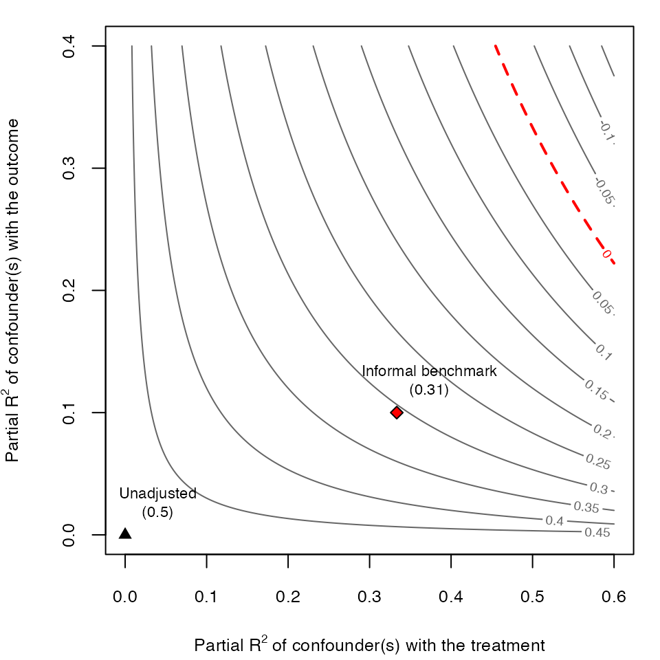
We can now plot the sensitivity contours with ovb_contour_plot() and add our informal benchmark with the numeric method of add_bound_to_contour(). The arguments label.bump.x and label.bump.y of these functions allow adjusting the position of the bound label in the plot.

# draws sensitivity contours
ovb_contour_plot(model.ydx,  
                 treatment = "D", 
                 lim = .6)

# adds informal benchmark 
add_bound_to_contour(r2dz.x = r2dx, 
                     r2yz.dx = r2yx.d, 
                     bound_value = informal_adjusted_estimate,
                     bound_label = "Informal benchmark")

As we can see, the results of the informal benchmark are different from what we expected. The informal benchmark point is still far away from zero, and this would lead an investigator to incorrectly conclude that an unobserved confounder \(Z\) “not unlike \(X\)” is not sufficient to explain away the observed effect. Moreover, this incorrect conclusion occurs despite correctly assuming that: (i) \(Z\) and \(X\) have the same strength of association with \(D\) and \(Y\); and, (ii) \(Z\) is independent of \(X\). Why does this happen?

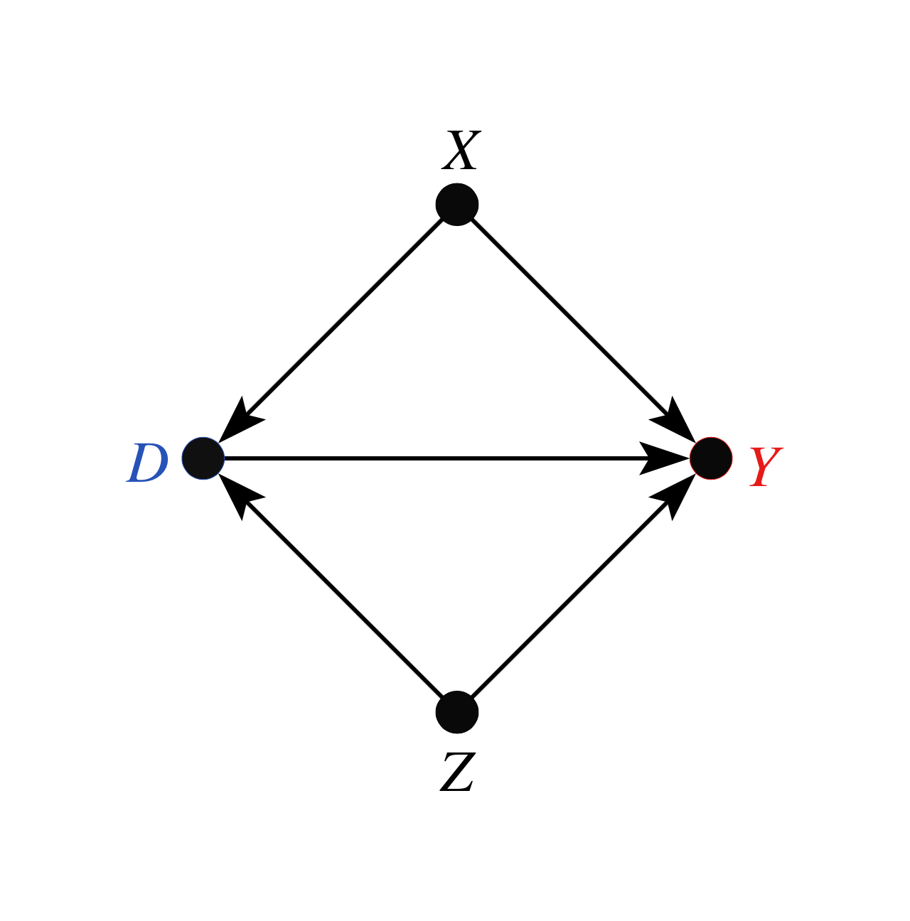
As explained in Section 6.1 of Cinelli and Hazlett (2020), there are two problems affecting informal benchmarks in this setting. First, we have to make an adjustment of baseline variance to be explained, since the sensitivity parameters consider the partial \(R^2\) of \(Z\) with the outcome, after taking into account what is already explained by \(X\). Second, consider the DAG of our structural model:

That is, although \(Z\) is marginally independent of \(X\), note that \(Z\) is not conditionally independent of \(X\), given \(D\), because \(D\) is a collider (Pearl, 2009). This distorts the observed quantities of \(X\) that are being used for benchmarking.

Formal bounds

Given the above considerations, we do not recommend using informal benchmarks for sensitivity analysis. We now show how to compute formal bounds. In sensemakr, you can use the function ovb_bounds().

# compute formal bounds
formal_bound <- ovb_bounds(model = model.ydx, 
                           treatment = "D", 
                           benchmark_covariates = "X", 
                           kd = 1, ky = 1)

In this function you specify the linear model being used (model.ydx), the treatment of interest (\(D\)), the observed variable used for benchmarking (\(X\)), and how stronger \(Z\) is in explaining treatment (kd) and outcome (ky) variation, as compared to the benchmark variable \(X\). We can now plot the proper bound against the informal benchmark.

# contour plot
ovb_contour_plot(model.ydx,  
                 treatment = "D",
                 lim = .6)

add_bound_to_contour(r2dz.x = r2dx, 
                     r2yz.dx = r2yx.d, 
                     bound_value = informal_adjusted_estimate,
                     bound_label = "Informal benchmark")

add_bound_to_contour(bounds = formal_bound,
                     bound_label = "Proper bound")

Note that, using the formal bounds, the researcher now reaches the correct conclusion that, an unobserved confounder \(Z\) similar to \(X\) is strong enough to explain away all the observed association. For further details, please see Sections 4.4 and 6.1 of Cinelli and Hazlett (2020).

References

Cinelli, C. Hazlett, C. (2020) “Making Sense of Sensitivity: Extending Omitted Variable Bias”. Journal of the Royal Statistical Society, Series B (Statistical Methodology). ( link )