This function performs sensitivity analysis to omitted variables as discussed in Cinelli and Hazlett (2020). It returns an object of
class sensemakr with several pre-computed sensitivity statistics for reporting.
After running sensemakr you may directly use the plot, print and summary methods in the returned object.
sensemakr(...)

# S3 method for class 'lm'
sensemakr(
  model,
  treatment,
  benchmark_covariates = NULL,
  kd = 1,
  ky = kd,
  q = 1,
  alpha = 0.05,
  r2dz.x = NULL,
  r2yz.dx = r2dz.x,
  bound_label = "Manual Bound",
  reduce = TRUE,
  ...
)

# S3 method for class 'fixest'
sensemakr(
  model,
  treatment,
  benchmark_covariates = NULL,
  kd = 1,
  ky = kd,
  q = 1,
  alpha = 0.05,
  r2dz.x = NULL,
  r2yz.dx = r2dz.x,
  bound_label = "Manual Bound",
  reduce = TRUE,
  ...
)

# S3 method for class 'formula'
sensemakr(
  formula,
  method = c("lm", "feols"),
  vcov = "iid",
  data,
  treatment,
  benchmark_covariates = NULL,
  kd = 1,
  ky = kd,
  q = 1,
  alpha = 0.05,
  r2dz.x = NULL,
  r2yz.dx = r2dz.x,
  bound_label = "",
  reduce = TRUE,
  ...
)

# S3 method for class 'numeric'
sensemakr(
  estimate,
  se,
  dof,
  treatment = "D",
  q = 1,
  alpha = 0.05,
  r2dz.x = NULL,
  r2yz.dx = r2dz.x,
  bound_label = "manual_bound",
  r2dxj.x = NULL,
  r2yxj.dx = r2dxj.x,
  benchmark_covariates = "manual_benchmark",
  kd = 1,
  ky = kd,
  reduce = TRUE,
  ...
)
Arguments
- ...
arguments passed to other methods.
- model
An
lmorfixestobject with the outcome regression.- treatment
A character vector with the name of the treatment variable of the model.
- benchmark_covariates
The user has two options: (i) character vector of the names of covariates that will be used to bound the plausible strength of the unobserved confounders. Each variable will be considered separately; (ii) a named list with character vector names of covariates that will be used, as a group, to bound the plausible strength of the unobserved confounders. The names of the list will be used for the benchmark labels. Note: for factor variables with more than two levels, you need to provide the name of each level as encoded in the
fixestmodel (the columns ofmodel.matrix).- kd
numeric vector. Parameterizes how many times stronger the confounder is related to the treatment in comparison to the observed benchmark covariate. Default value is
1(confounder is as strong as benchmark covariate).- ky
numeric vector. Parameterizes how many times stronger the confounder is related to the outcome in comparison to the observed benchmark covariate. Default value is the same as
kd.- q
percent change of the effect estimate that would be deemed problematic. Default is
1, which means a reduction of 100% of the current effect estimate (bring estimate to zero). It has to be greater than zero.- alpha
significance level.
- r2dz.x
hypothetical partial R2 of unobserved confounder Z with treatment D, given covariates X.
- r2yz.dx
hypothetical partial R2 of unobserved confounder Z with outcome Y, given covariates X and treatment D.
- bound_label
label to bounds provided manually in
r2dz.xandr2yz.dx.- reduce
should the bias adjustment reduce or increase the absolute value of the estimated coefficient? Default is
TRUE.- formula
an object of the class
formula: a symbolic description of the model to be fitted.- method
the default is
lm. This argument can be changed to estimate the model usingfeols. In this case the formula needs to be written so it can be estimated withfeolsand the package needs to be installed.- vcov
the variance/covariance used in the estimation when using
feols. Seevcov.fixestfor more details. Defaults to "iid".- data
data needed only when you pass a formula as first parameter. An object of the class
data.framecontaining the variables used in the analysis.- estimate
Coefficient estimate.
- se
standard error of the coefficient estimate.
- dof
residual degrees of freedom of the regression.
- r2dxj.x
partial R2 of covariate Xj with the treatment D (after partialling out the effect of the remaining covariates X, excluding Xj).
- r2yxj.dx
partial R2 of covariate Xj with the outcome Y (after partialling out the effect of the remaining covariates X, excluding Xj).
Value
An object of class sensemakr, containing:
-
info A
data.framewith the general information of the analysis, including the formula used, the name of the treatment variable, parameter values such asq,alpha, and whether the bias is assumed to reduce the current estimate.-
sensitivity_stats A
data.framewith the sensitivity statistics for the treatment variable, as computed by the functionsensitivity_stats.-
bounds A
data.framewith bounds on the strength of confounding according to some benchmark covariates, as computed by the functionovb_bounds.
References
Cinelli, C. and Hazlett, C. (2020), "Making Sense of Sensitivity: Extending Omitted Variable Bias." Journal of the Royal Statistical Society, Series B (Statistical Methodology).
See also
The function sensemakr is a convenience function. You may use the other sensitivity functions of the package directly, such as the functions for sensitivity plots
(ovb_contour_plot, ovb_extreme_plot) the functions for computing bias-adjusted estimates and t-values (adjusted_estimate, adjusted_t),
the functions for computing the robustness value and partial R2 (robustness_value, partial_r2), or the functions for bounding the strength
of unobserved confounders (ovb_bounds), among others.
Examples
# loads dataset
data("darfur")
# runs regression model
model <- lm(peacefactor ~ directlyharmed + age + farmer_dar + herder_dar +
pastvoted + hhsize_darfur + female + village, data = darfur)
# runs sensemakr for sensitivity analysis
sensitivity <- sensemakr(model, treatment = "directlyharmed",
benchmark_covariates = "female",
kd = 1:3)
# short description of results
sensitivity
#> Sensitivity Analysis to Unobserved Confounding
#>
#> Model Formula: peacefactor ~ directlyharmed + age + farmer_dar + herder_dar +
#> pastvoted + hhsize_darfur + female + village
#>
#> Null hypothesis: q = 1 and reduce = TRUE
#>
#> Observed Estimates of ' directlyharmed ':
#> Coef. estimate: 0.09732
#> Standard Error: 0.02326
#> t-value: 4.18445
#>
#> Sensitivity Statistics:
#> Partial R2 of treatment with outcome: 0.02187
#> Robustness Value, q = 1 : 0.13878
#> Robustness Value, q = 1 alpha = 0.05 : 0.07626
#>
#> For more information, check summary.
# long description of results
summary(sensitivity)
#> Sensitivity Analysis to Unobserved Confounding
#>
#> Model Formula: peacefactor ~ directlyharmed + age + farmer_dar + herder_dar +
#> pastvoted + hhsize_darfur + female + village
#>
#> Null hypothesis: q = 1 and reduce = TRUE
#> -- This means we are considering biases that reduce the absolute value of the current estimate.
#> -- The null hypothesis deemed problematic is H0:tau = 0
#>
#> Observed Estimates of 'directlyharmed':
#> Coef. estimate: 0.0973
#> Standard Error: 0.0233
#> t-value (H0:tau = 0): 4.1844
#>
#> Sensitivity Statistics:
#> Partial R2 of treatment with outcome: 0.0219
#> Robustness Value, q = 1: 0.1388
#> Robustness Value, q = 1, alpha = 0.05: 0.0763
#>
#> Verbal interpretation of sensitivity statistics:
#>
#> -- Partial R2 of the treatment with the outcome: an extreme confounder (orthogonal to the covariates) that explains 100% of the residual variance of the outcome, would need to explain at least 2.19% of the residual variance of the treatment to fully account for the observed estimated effect.
#>
#> -- Robustness Value, q = 1: unobserved confounders (orthogonal to the covariates) that explain more than 13.88% of the residual variance of both the treatment and the outcome are strong enough to bring the point estimate to 0 (a bias of 100% of the original estimate). Conversely, unobserved confounders that do not explain more than 13.88% of the residual variance of both the treatment and the outcome are not strong enough to bring the point estimate to 0.
#>
#> -- Robustness Value, q = 1, alpha = 0.05: unobserved confounders (orthogonal to the covariates) that explain more than 7.63% of the residual variance of both the treatment and the outcome are strong enough to bring the estimate to a range where it is no longer 'statistically different' from 0 (a bias of 100% of the original estimate), at the significance level of alpha = 0.05. Conversely, unobserved confounders that do not explain more than 7.63% of the residual variance of both the treatment and the outcome are not strong enough to bring the estimate to a range where it is no longer 'statistically different' from 0, at the significance level of alpha = 0.05.
#>
#> Bounds on omitted variable bias:
#>
#> --The table below shows the maximum strength of unobserved confounders with association with the treatment and the outcome bounded by a multiple of the observed explanatory power of the chosen benchmark covariate(s).
#>
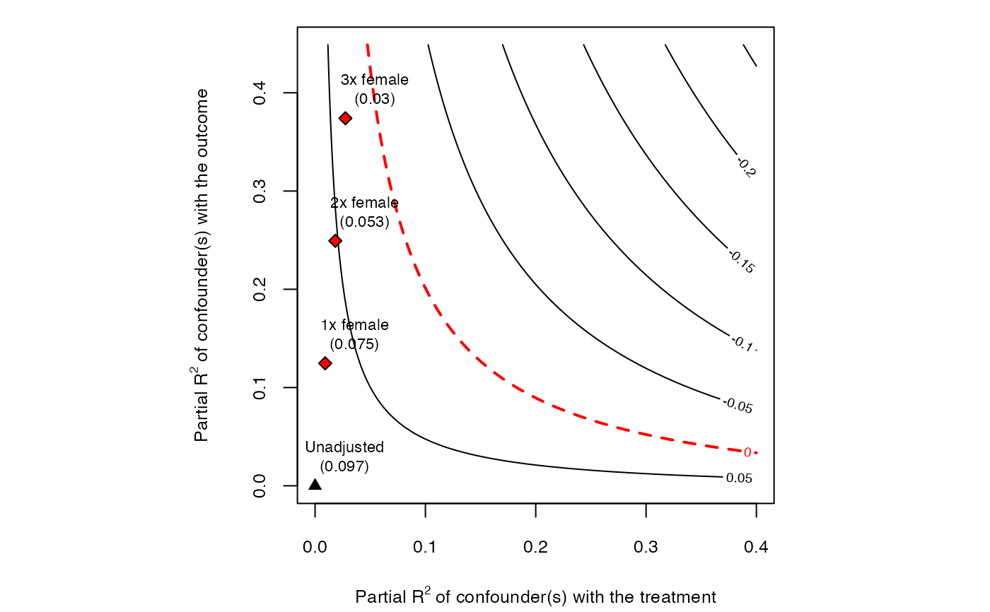
#> Bound Label R2dz.x R2yz.dx Treatment Adjusted Estimate Adjusted Se
#> 1x female 0.0092 0.1246 directlyharmed 0.0752 0.0219
#> 2x female 0.0183 0.2493 directlyharmed 0.0529 0.0204
#> 3x female 0.0275 0.3741 directlyharmed 0.0304 0.0187
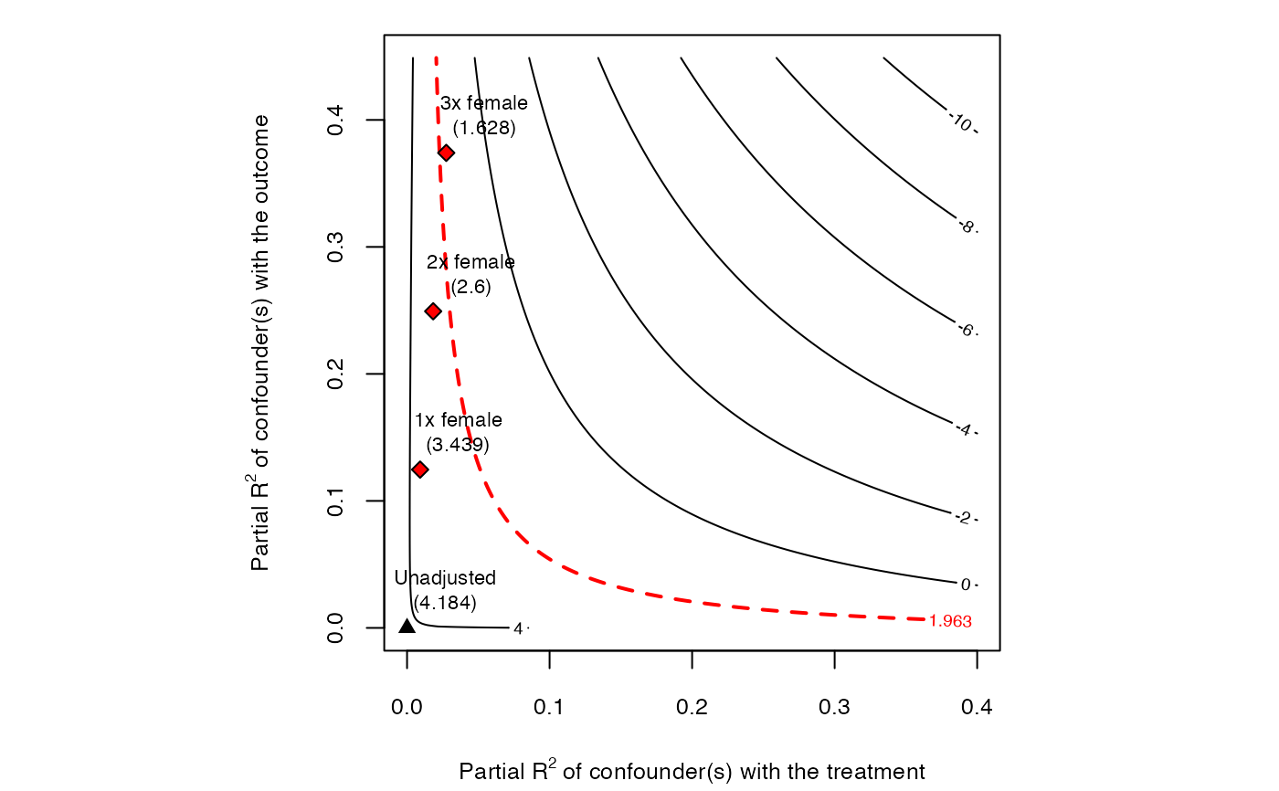
#> Adjusted T Adjusted Lower CI Adjusted Upper CI
#> 3.4389 0.0323 0.1182
#> 2.6002 0.0130 0.0929
#> 1.6281 -0.0063 0.0670
# plot bias contour of point estimate
plot(sensitivity)
 # plot bias contour of t-value
plot(sensitivity, sensitivity.of = "t-value")
# plot bias contour of t-value
plot(sensitivity, sensitivity.of = "t-value")
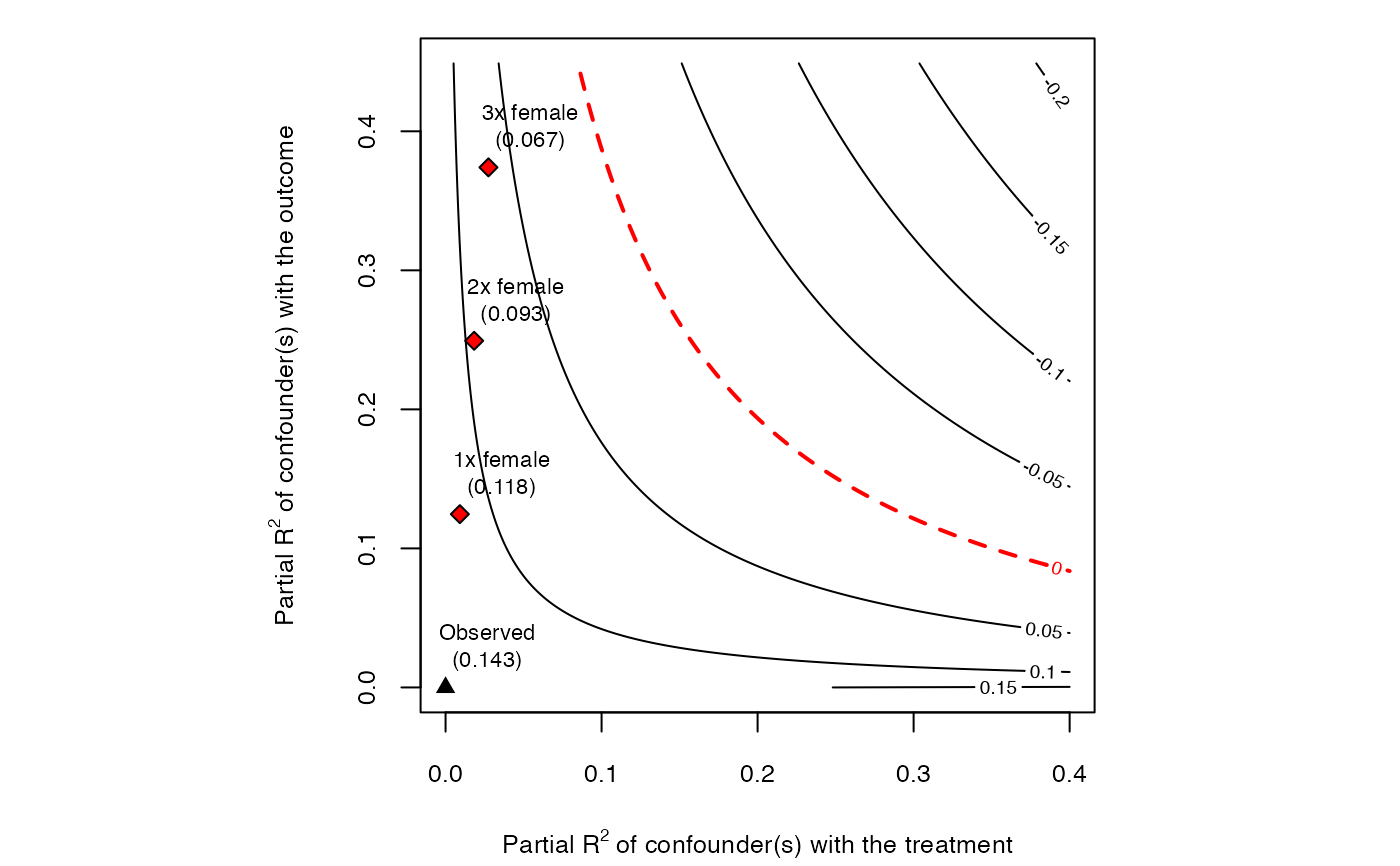
 # plot bias contour of lower limit of CI
plot(sensitivity, sensitivity.of = "lwr")
# plot bias contour of lower limit of CI
plot(sensitivity, sensitivity.of = "lwr")
 # plot bias contour of upper limit of CI
plot(sensitivity, sensitivity.of = "upr")
# plot bias contour of upper limit of CI
plot(sensitivity, sensitivity.of = "upr")
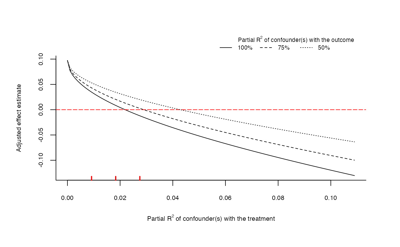
 # plot extreme scenario
plot(sensitivity, type = "extreme")
# plot extreme scenario
plot(sensitivity, type = "extreme")
 # latex code for sensitivity table
ovb_minimal_reporting(sensitivity)
#> \begin{table}[!h]
#> \centering
#> \begin{tabular}{lrrrrrr}
#> \multicolumn{7}{c}{Outcome: \textit{peacefactor}} \\
#> \hline \hline
#> Treatment: & Est. & S.E. & t-value & $R^2_{Y \sim D |{\bf X}}$ & $RV_{q = 1}$ & $RV_{q = 1, \alpha = 0.05}$ \\
#> \hline
#> \textit{directlyharmed} & 0.097 & 0.023 & 4.184 & 2.2\% & 13.9\% & 7.6\% \\
#> \hline
#> df = 783 & & \multicolumn{5}{r}{ \small \textit{Bound (1x female)}: $R^2_{Y\sim Z| {\bf X}, D}$ = 12.5\%, $R^2_{D\sim Z| {\bf X} }$ = 0.9\%} \\
#> \end{tabular}
#> \end{table}
# latex code for sensitivity table
ovb_minimal_reporting(sensitivity)
#> \begin{table}[!h]
#> \centering
#> \begin{tabular}{lrrrrrr}
#> \multicolumn{7}{c}{Outcome: \textit{peacefactor}} \\
#> \hline \hline
#> Treatment: & Est. & S.E. & t-value & $R^2_{Y \sim D |{\bf X}}$ & $RV_{q = 1}$ & $RV_{q = 1, \alpha = 0.05}$ \\
#> \hline
#> \textit{directlyharmed} & 0.097 & 0.023 & 4.184 & 2.2\% & 13.9\% & 7.6\% \\
#> \hline
#> df = 783 & & \multicolumn{5}{r}{ \small \textit{Bound (1x female)}: $R^2_{Y\sim Z| {\bf X}, D}$ = 12.5\%, $R^2_{D\sim Z| {\bf X} }$ = 0.9\%} \\
#> \end{tabular}
#> \end{table}